Welcome to my Mat 301 Calculus I site!

Quiz 1

Sample Questions

---

---

Question 1

Using differentials find the first order (linear) approximation of  using 

Answer to Question 1:      .

Video on how to solve Question 1.

 

---

---

Question 2

Using differentials find the first order (linear) approximation of  using .


Note.

Answer to Question 2:      .

Video on how to solve Question 2

 

Graph showing geometry of the linear approximation carried out in Question 2 above.

 

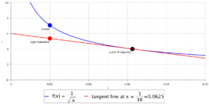
The following Maple commands will find the linear approximation for Question 2 and create the graph shown above.  You can copy and paste the following commands into Maple.

 with(plots):
f := x -> 1/sqrt(x);
x0 := 1/16;
x_app := 0.02;
xStart := 0:
xFinish := 0.1:
yStart := 0:
yEnd := 10:
TangentLine := (f, x0, x) -> D(f)(x0)*(x - x0) + f(x0):
"tangent line equation y  = mx +b of f(x) at x = x0 ";
evalf(TangentLine(f, x0, x));
"linear approximation of f(x_app) ";
evalf(TangentLine(f, x0, x_app));
"exact actual value of f(x_app)";
f(x_app);
"x intercept of tangent line equation";
solve(evalf(TangentLine(f, x0, x)), x);
plotA := plot([f(x), TangentLine(f, x0, x)], 
  x = xStart .. xFinish,
  y = yStart .. yEnd, gridlines, 
  color = [blue, red], 
  legend = [typeset("  f(x) = ", f(x), "    "), 
    typeset("  tangent line at x = ", x0, "=", evalf[3](x0))],
  legendstyle = [font = ["HELVETICA", 30], location = bottom],
  thickness = 4, size = [0.7, 0.5]):
plotB := pointplot([[x_app, f(x_app)], 
  [x_app, TangentLine(f, x0, x_app)], [x0, f(x0)]], 
  color = [blue, red, black], 
  symbol = solidcircle, symbolsize = 20):
plotC := textplot([x_app, 0.97*f(x_app), "actual"], 
  align = {'below', 'left'}):
plotD := textplot([x_app, 0.97*TangentLine(f, x0, x_app),
  "approximation"], align = {'below', 'left'}):
plotE := textplot([x0, 0.97*TangentLine(f, x0, x0), 
  "point of tangency"], align = {'below', 'left'}):
display({plotA, plotB, plotC, plotD, plotE});

 

---

---

Question 3

Below is shown the graph of f(x). 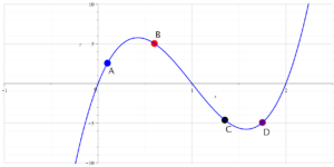 By inspection, meaning, just by looking at the graph, answer the following questions.

Put the best answer: A, B, C, or D, on the line:

Put the best answer:  INCREASING or DECREASING on the line:

At the point A the function  is: 

At the point B the function  is: 

At the point C the function  is: 

At the point D the function  is: 

Put the best answer:  UP or DOWN on the line:

At the point A the function  is concave: 

At the point B the function  is concave: 

At the point C the function  is concave: 

At the point D the function  is concave: 

Video on how to solve Question 3.

 

The following Maple commands were used to produce the graph shown above (Question 3).  You can copy and paste the following code into Maple.

 with(plots):
f := x -> 15*x*(x - 1)*(x - 2);
xA := 0.1;
xB := 0.6;
xC := 1.35;
xD := 1.75;
xStart := -1:
xFinish := 2.5:
yStart := -10:
yEnd := 10:
plotMain := plot([f(x)], x = xStart .. xFinish, 
  y = yStart .. yEnd, gridlines, color = [blue], 
  size = [0.7, 0.5], thickness = 4):
plotP := pointplot([[xA, f(xA)], [xB, f(xB)], [xC, f(xC)], 
  [xD, f(xD)]], color = [blue, red, black, purple], 
  symbol = solidcircle, symbolsize = 20):
plotTA := textplot([xA, 0.9*f(xA), "A", 
  font = ["HELVETICA", 35]], align = {'below', 'right'}):
plotTB := textplot([xB, 1.1*f(xB), "B", 
  font = ["HELVETICA", 35]], align = {'above', 'right'}):
plotTC := textplot([xC, 1.1*f(xC), "C", 
  font = ["HELVETICA", 35]], align = {'below', 'right'}):
plotTD := textplot([xD, 1.1*f(xD), "D", 
  font = ["HELVETICA", 35]], align = {'below', 'right'}):
display({plotP, plotTA, plotTB, plotTC, plotTD, plotMain}); 

 

---

---