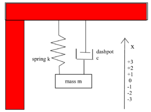
Let $x(t)$ measure the distance the mass of a damped harmonic oscillator is from its equilibrium position at time $t$. Note. The equilibrium position is assumed to be at $x = 0$. See image below.
The damped harmonic oscillator can be modeled by the following Differential Equation (DE) which we present as an Initial Value Problem (IVP) since we are including Initial Conditions (IC):
$ m \ddot{x} + c\dot{x} + kx = 0$
$ x(0) = x_0, \ \ \dot{x}(0) = v_0 $
$m =$ mass, $c =$ the damping constant, and $k =$ the spring constant, with $m, c, k > 0$.
We divide the DE by $m$ to get the equivalent DE:
$ \ddot{x} + \frac{c}{m}\, \dot{x} + \frac{k}{m}\, x = 0$
$x(0) = x_0, \ \ \dot{x}(0) = v_0 $
which is easier to work with. If we want, we can think of $c$ as representing $\frac{c}{m}$ and $k$ as representing $\frac{k}{m}$. With these substitutions the DE becomes:
$ \ddot{x} + c\dot{x} + k x = 0$
$ x(0) = x_0, \ \ \dot{x}(0) = v_0 $
The letters $c$ and $k$ appearing in the differential equation
$$ \ddot{x} + c\dot{x} + k x = 0$$
are called parameters. Sometimes the values of parameters appearing in a DE can be measured directly. For example, if we go back to our first DE for the damped harmonic oscillator:
$$m \ddot{x} + c\dot{x} + k x = 0$$
the parameter $m$, which is the mass, could be found by putting the mass on a scale and weighing it. However, often it is the case that there is no easy way to directly measure parameters. Instead their values need to be estimated from data, the data being measurements made on the entire system.
For example, with the damped harmonic oscillator we might have measured the position of the mass at several different times. This would result in our having a set of data points. One data point $(t, x)$ for each (time, position) measurement:
$$(t_i, x_i) \ \text{ with } \ i = 0, 1, 2, \ldots, n$$
This project. In this project we will estimate the parameters $c$ and $k$ of the DE
$ \ddot{x} + c\dot{x} + k x = 0$
$ x(0) = x_0, \ \ \dot{x}(0) = v_0 $
from data points of the form $(t_i, x_i)$ with $i = 0, 1, 2, \ldots, n$.
Note. The Python program embedded below will generate simulated data for us.
Method of Parameter Estimation.
We will think of the parameters that we want to estimate, the $c$ and the $k$, as “living” in parameter space which consists of points $(c, k)$.
At each point $(c, k)$ in parameter space we can solve the differential equation
$ \ddot{x} + c\dot{x} + k x = 0$
$ x(0) = x_0, \ \ \dot{x}(0) = v_0 $
We write the solution as $x(c,k,t)$, instead of as just $x(t)$, to emphasize that the solution is a function of of the parameters $c$ and $k$.
We want to find the $(c, k)$ which minimizes the distance between $x(c,k,t)$ and the data. We measure this distance using the Sum of the Squared Errors (SSE).

We can think of the DE’s solution, $x(c, k, t)$, as predicting the position of the mass at time $t.$
We calculate $x(c, k, t)$ using the Euler method.
The data point $(t_i, x_i)$ is the actual or true position of the mass at time $t$. The $i^{th}$ error is the difference between where $x$ predicted the mass would be at time $t_i$, which is $x(c, k, t_i)$ and were the mass actually is at time $ t_i$, which is $x_i$.
For each $i, \ i = 0, 1, 2, \ldots, n$, the error is
$$\epsilon_i = x(c,k, t_i) – x_i$$
and the squared error is
$$\epsilon_{i}^{2} = \left(x(c,k, t_i) – x_i\right)^2$$
Finally, to get the SSE, we sum up the squared errors
$$ SSE(c, k) = \sum_{i=0}^{n} \left(x(c,k, t_i) – x_i\right)^2$$
Note. The SSE is a a function of $(c,k)$, hence the notation $SSE(c,k)$.
Keep in mind, each time the computer calculates the $SSE$ at $(c, k)$ the computer has run the Euler method algorithm to calculate the Euler points which approximate $x(c, k, t)$. Then the computer uses interpolation to estimate each $x(c, k, t_i)$. For more about interpolation see the notes at the bottom of this page.
Note about SSE. For some general information on the SSE in the context of regression see:
https://mccarthymat150.commons.gc.cuny.edu/units-16/17-correlation-and-regression/
Next, we need an efficient algorithm to find the $(c, k)$ which minimizes $SSE(c, k)$. The algorithm we will use is called the Gradient Descent Algorithm (GDA).
Note about GDA. For some general information about the GDA see:
https://mccarthymat501.commons.gc.cuny.edu/gradient-descent-algorithm-gda/
The following Python 3 program uses entirely numerical methods to estimate the parameters $(c, k).$ It solves the harmonic oscillator differential equation using Euler’s Method. It calculates the gradients used in the GDA numerically.
Outline of how the program works. You can accept the defaults, or you can chose values for $c$ and $k$ to be used in the differential equation model. Similarly, you can accept the defaults, or you can choose a different starting point $(c_0, k_0)$ for the GDA. Another important variable you can change is called
$\text{ GDAiterations }$
its default value is 200, meaning the GDA should iterate itself 200 times.
The program then uses the Euler method to numerically solve the differential equation for the chosen values of $c$ and $k$. It uses that solution to generate data with noise in it using a random number generator. The idea is to simulate the sorts of measurements you would get if you were working with a physical damped harmonic oscillator, like in a physics lab.
The program applies the GDA to the $SSE(c, k)$ to estimate the parameters $(c, k)$.
The program outputs the GDA estimate for $(c, k)$ (which it reports as c/m and k/m) as well as the SSE for that estimate and some additional information:
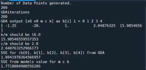
Then, if the option $\text{ Do3DandContourPlot = 1 }$ the program will output two graphs.
Note. The most time consuming part of the program is doing the calculations to produce these graphs. As these calculations are done, Python outputs what percent of the calculations are left to do.
The first is the SSE(c,k) surface with the GDA path superimposed on it. The surface height and GDA path height are scaled by log 10. This is to prevent the huge values of the SSE at some locations from making it impossible to see, in the graph, the details at locations were the SEE is near its minimum. See image below:
Note. All images were produced by the source code embedded at the bottom of this page.
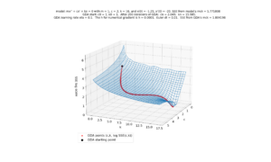
Note that in Python, the above graph can be rotated interactively:
The second graph is the SSE(c,k) surface, again scaled by log 10, shown as a two dimensional contour map. The contours being the level curves of the surface. The GDA path is superimposed on it. See image below:

Note that in Python, sections of the graph can be magnified using the magnifying glass tool. That tool is at the top of the graph window. See video and image below:
Video of Contour Map showing SSE(c,k) and the GDA path in (c, k) space.

In the above image, which is a zoomed in version of the previous image, we see the last points produced by the GDA. Notice how the GDA nicely gets us close to the minimum SSE (the center of that blue polygonal shape) but then starts to zigzag a little. That zigzagging behavior is a common artifact of GDA. To counter that, I have our GDA output the $(c, k)$ estimate as the average of the last two GDA points.
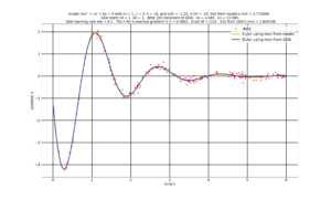
After the optional 3D and contour graphs, the program will produce a graph showing the data points $(t_i, x_i)$ (red dots) together with the solution $(t, x(t))$ with x(t) being numerically solved by applying the Euler method to the initial choice of c, k, i.e., from the model (yellow line) and from the final GDA estimate of c, k (blue line). See graph below.
The program will finally produce a video of the above graph, showing the evolution the solution x(c,k, t) as the GDA updates its estimates of (c, k). See video below.
Note. Unlike the static graph above, that the video does not graph $x(c, k, t)$ for the final estimate of $(c, k)$. Recall that the final estimate of $(c,k)$ comes from the average of the final two GDA estimates for $(c, k)$. We take that average in order to compensate for the zigzagging that tends to happen at the end of the GDA.
In the video below, the up and down motion of the $x(c,k,t)$ (blue) starting at GDA iteration 170 is due to the GDA estimates of $(c, k)$ zigzagging. This zigzagging can be seen towards the end of the video of the contour map (embedded a few paragraphs above).
# Written by Chris McCarthy March 2022
# numerically finds the parameters c,k that best fit
# the harmonic oscillator mx'' +cx' + k = 0 with x(0) = x0 and x'(0) = v0
# to data generated by Python
# m = 1 ----- m should be 1
#=========================================== Graphics Note
# update anaconda then in Spyder Pref iPython Graphics Backend InLine
#=========================================== Online Compiling Note
# https://trinket.io/features/python3 python online
#=========================================== usual Python packages
import numpy as np
#from mpl_toolkits import mplot3d
from matplotlib import pyplot as plt
plt.rcParams.update({'font.size': 22})
#=================== (global variables) ODE IC
x0 = -1.25
v0 = -20
#=================== (global variables) ODE params
m = 1 # do not change m
c = 2 # you can change c and or k
k = 16
#======================== (global variables) for GDA starting point (m, c, k)
m0 = m/m # DO NOT CHANGE m0
c0 = 1 # you can change c0 and or k0
k0 = 1
GDAiterations = 200 # How many iterations of GDA to do
#=================== (global variables) time t start and stop
t0 = 0 #time start
tf = 6 #time stop
#=================== (global variables) Euler time step
dt = 0.01 # for Euler
# ================= (global variables) GDA learning rate and numerical gradient
eta = .1 # for GDA learning rate
h = 0.0001 # for numerical gradient
#=================== (global variables) for Euler Method
En = np.ceil((tf-t0)/dt).astype(int)+1 # how many Euler points to do
ET = np.linspace(t0, tf, En) # Euler tn time values
# ======================= what to plot
Do3DandContourPlot = 1 # 1 = do the 3D plot and Contour Plots
#================================== (global variables) for contour map
ckGrid = 50 # SSE will be calculated at (c, k) at contourGrid x contourGrid
contourLevels = 100 # how many levels to show in the contour map
legendLocationContour = 4 # 1 upperRight 2 upperLeft 3 lowerLeft 4 lowerRight
#================================== (global variables) Python generated data points
NumberOfDataPoints = 200 # number of data points to generate
SpreadOfDataPoints = 0.1 # was 0.02
#================================== (global variables) Python generated data points
np.random.seed(5) # will create the same random sequence every time
# you can change 200 to any pos integer
# used to generate random data points
# ============================ Functions
def ODE(x,v,m,c,k): #mx'' + cx' + kx = 0 ODE as Vector Field
    return [v, -(c/m)*v - (k/m)*x]
# Outputs x value of Euler points
def EulerX(fn, x0, v0, m, c, k):
    n = np.ceil((tf-t0)/dt).astype(int)+1
    EPX = np.empty(n, dtype=float)
    EPV = np.empty(n, dtype=float)
    EPX[0]=x0
    EPV[0]= v0
    for i in range(0,n-1):
        EPX[i+1]=EPX[i]+ fn(EPX[i],EPV[i],m,c,k)[0]*dt
        EPV[i+1]=EPV[i]+ fn(EPX[i],EPV[i],m,c,k)[1]*dt
    return EPX
# converts Euler tn and Euler xn to function using linear interpolation
def LinearInterpolation(npInArray, npOutArray, InValue):
    a = np.where(npInArray<=InValue)[0][-1]
    b = np.where(npInArray>=InValue)[0][0]
    if npInArray[a] == InValue:
        returnValue = npOutArray[a]
    else:
        slope = (npOutArray[b] - npOutArray[a])/(npInArray[b] - npInArray[a])
        returnValue = npOutArray[a] + slope *(InValue - npInArray[a])
    return(returnValue)
# =============================== Following Code Generates noisy data
# correspoding to mx'' + cx' + ks = 0
#=============================================================
UseRandomData = 1
if UseRandomData == 1:
    EXX = np.array(EulerX(ODE, x0, v0, m,c,k )) # Euler from model's mck
    #np.random.seed(1)
    DataTT = np.random.uniform(t0, tf, NumberOfDataPoints)
    DataXX = np.empty(NumberOfDataPoints, dtype=float)
    for i in range(0, NumberOfDataPoints):
        DataXX[i] = LinearInterpolation( ET, EXX, DataTT[i] ) + SpreadOfDataPoints*np.random.randn()
    dataT = DataTT
    dataX = DataXX
    print('Number of Data Points generated.')
    print(NumberOfDataPoints)
n = len(dataT)
# ============================ More Functions
# Outputs Sum of the Squared Errors (distance from Euler to Data)
def SSE(x0,v0,m,c,k):
    EPX = np.array(EulerX(ODE, x0, v0, m,c,k ))
    EPXatTi = np.empty(n, dtype=float)
    for i in range(0, n):
        EPXatTi[i] = LinearInterpolation(ET, EPX, dataT[i] )
    return(np.sum((EPXatTi-dataX)**2))
# for use with 3D plotting. Input mesh c and k, output mesh SSE
def SSE_plot(c,k):
    ArrayShape = np.shape(c)
    ArrayOut = np.empty(ArrayShape, dtype=float)
    for cols in range(0, ArrayShape[1]):
        percentLeft = np.round(100*(1 - cols/ArrayShape[1]))
        print(f'{percentLeft} percent of calculations remaining')
        for rows in range(0, ArrayShape[0]):
            EPX = np.array(EulerX(ODE, x0, v0, m,c[rows][cols],k[rows][cols] ))
            EPXatTi = np.empty(n, dtype=float)
            for i in range(0, n):
                EPXatTi[i] = LinearInterpolation(ET, EPX, dataT[i] )
            ArrayOut[rows][cols] = np.sum((EPXatTi-dataX)**2)
    return(ArrayOut)
# for use with 2d contour plotting. Input vector c and k, output vector SSE
def SSE_plot_pts(c,k):
    ArrayShape = len(c)
    ArrayOut = np.empty(ArrayShape, dtype=float)
    for j in range(0, ArrayShape):
        EPX = np.array(EulerX(ODE, x0, v0, m,c[j],k[j]))
        EPXatTi = np.empty(n, dtype=float)
        for i in range(0, n):
            EPXatTi[i] = LinearInterpolation(ET, EPX, dataT[i] )
        ArrayOut[j] = np.sum((EPXatTi-dataX)**2)
    return(ArrayOut)
# Calculates numerical gradient in c,k direction
def GRADmck2(x,v,m,c,k):
    ssec = (SSE(x,v,m,c+h,k)-SSE(x,v,m,c-h,k))/(2*h)
    ssek = (SSE(x,v,m,c,k+h)-SSE(x,v,m,c,k-h))/(2*h)
    return np.array( [0, 0, 0, ssec, ssek])
# Does GDA algorithm
def GDAmck2(x,v,m,c,k, its):
    gda_p = np.empty((its, 5), dtype=float)
    p = np.array([x,v,m,c,k])
    gda_p[0,:] = p
    for i in range(1, its):
        g = GRADmck2(p[0], p[1],p[2],p[3],p[4])
        ng = np.sqrt(g[0]**2 + g[1]**2 + g[2]**2 + g[3]**2 + g[4]**2)
        if ng > 1:
            p = p - (eta/ng)*g #new
        else:
            p = p - eta*g #original
        gda_p[i, :] = p #new
    return gda_p
# =============================================================================
# Print how many iterations in the GDA is being used
print('GDAiterations')
print(GDAiterations)
#======================== Call GDA and print results
b2 = GDAmck2(x0, v0, m0, c0, k0, GDAiterations)
# to get the final (c,k) of GDA average the last two GDA points
b = .5*(b2[GDAiterations-1] + b2[GDAiterations-2])
print('GDA output [x0 v0 m c k] as b[i] i = 0 1 2 3 4')
print(b)
#print(b2)
print(f'k/m should be {k/m}')
print(b[4]/b[2])
print(f'c/m should be {c/m}')
print(b[3]/b[2])
print("SSE for (b[0], b[1], b[2], b[3], b[4]) from GDA")
SSE_from_GDA = SSE(b[0], b[1], b[2], b[3], b[4])
print(SSE_from_GDA)
print('SSE from models value for m c k')
SSE_from_model = SSE(x0,v0, m, c, k)
print(SSE_from_model)
# =================================================================
# graphing part of program
TitleString = f'model: mx\'\' + cx\' + kx = 0 with m = {m}, c = {c}, k = {k},\
 and x({t0}) = {x0}, x\'({t0}) = {v0}.\
 SSE from model\'s mck = {np.around(SSE_from_model, decimals=6) } \n \
 GDA start: c0 = {c0}, k0 = {k0}. \
 After {GDAiterations} iterations of GDA: \
 cn = {np.round(b[3]/b[2], 3)}, \
 kn = {np.round(b[4]/b[2], 3)}. \n \
 GDA learning rate eta = {eta}. \
 The h for numerical gradient is h = {h}. \
 Euler dt = {dt}. \
 SSE from GDA\'s mck = {np.around(SSE_from_GDA, decimals=6)}'
cc = b2[:, 3] # vector of c found from GDA
kk = b2[:, 4] # vector of k found from GDA
# ========================= range of (c,k) points found during GDA
cmin = np.min(b2[:,3])
cmax = np.max(b2[:,3])
kmin = np.min(b2[:,4])
kmax = np.max(b2[:,4])
# ========================= print range of (c,k)
print('c min max')
print(cmin)
print(cmax)
print('k min max')
print(kmin)
print(kmax)
# =============================================== 3d graph and contour plot
if (Do3DandContourPlot == 1):
    ccon = np.arange(cmin -1, cmax+1, (cmax - cmin)/ckGrid) # was 200
    kcon = np.arange(kmin - 1, kmax + 1, (kmax - kmin)/ckGrid) # was 200
    Xc, Yc = np.meshgrid(ccon, kcon) # backwards notation
    Zc = SSE_plot(Xc,Yc)
# 3DPlot
    fig = plt.figure(figsize = (12,10))
    ax = plt.axes(projection='3d')
    Z10 = np.log10(Zc)
    sse_ck = np.log10(SSE_plot_pts(cc,kk)) # use log scale for GDA trajectory
    surf = ax.plot_wireframe(Xc, Yc, Z10, cmap = plt.cm.cividis)
    ax.scatter(cc, kk, sse_ck, c = 'r', s = 50, label = 'GDA points (c,k, log SSE(c,k))')
    ax.scatter(cc[0], kk[0], sse_ck[0], c = 'black', s = 200, label = 'GDA starting point')
    # plot_surface or plot_wireframe can used
    ax.set_xlabel('c', labelpad=20)
    ax.set_ylabel('k', labelpad=20)
    ax.set_zlabel('SSE log scale', labelpad=20)
    #fig.colorbar(surf, shrink=0.5, aspect=8) # to put color bar next to plot
    leg = ax.legend(loc=3)
    plt.title(TitleString, fontsize = 20) # was 18
    plt.show()
# contour plot
# legend 1 upleft 2 upright 3 lowleft 4 lowright
    ToColor = 20
    ccStart = cc[0:ToColor]
    kkStart = kk[0:ToColor]
    ccEnd = cc[(GDAiterations-ToColor):(GDAiterations-1)]
    kkEnd = kk[(GDAiterations-ToColor):(GDAiterations-1)]
    # to plot using log scale
    Zc = np.log10(Zc)
    fig, ax = plt.subplots()
    ax.plot(cc, kk, 'o', color = 'r', label = 'GDA points (c,k)')
    ax.plot(cc, kk, 'y-',linewidth=2.0, label = 'GDA path')
    ax.plot(ccStart, kkStart, 'o', color = 'g', label = 'GDA starting points (c,k)')
    ax.plot(ccEnd, kkEnd, 'o', color = 'b', label = 'GDA ending points (c,k)')
    cp = ax.contour(Xc, Yc, Zc, levels = contourLevels)
    fig.colorbar(cp) # Add a colorbar to a plot
    ax.set_title('Filled Contours Plot')
    ax.set_xlabel('c \n Contour lines drawn at log SSE')
    ax.set_ylabel('k')
    leg = ax.legend(loc=legendLocationContour)
    plt.title(TitleString, fontsize = 20) # was 18
    plt.show()
# ===============================================================
# Plot data points and x(t) actual and with estimated parameters
# ======================= Calculate Euler Points from GDA and Models mck
x0 = b[0]
v0 = b[1]
mGDA = b[2]
cGDA = b[3]
kGDA = b[4]
EulerFromGDA = np.array(EulerX(ODE, x0, v0, mGDA,cGDA,kGDA )) # Euler from GDA
EX = np.array(EulerX(ODE, x0, v0, m,c,k )) # Euler from model's mck
# =============================================================================
fig, ax = plt.subplots()
ax.plot(dataT, dataX, 'o',color = 'r', label = 'data')
ax.plot(ET, EX, 'y-',linewidth=5.0, label = 'Euler using mck from model') # plot Euler from model's mck
ax.plot(ET, EulerFromGDA, 'b-',linewidth=3.0, label = 'Euler using mck from GDA') # plot Euler from GDA
#ax.axis('equal')
leg = ax.legend()
plt.grid(linewidth='3', color='black')
plt.title(TitleString, fontsize = 20) # was 18
ax.set_xlabel('time t')
ax.set_ylabel('position x')
plt.show()
#================================= animation video
import matplotlib.animation as animation
bb = b2[0]
x0 = bb[0]
v0 = bb[1]
mGDA = bb[2]
cGDA = bb[3]
kGDA = bb[4]
EulerFromGDA = np.array(EulerX(ODE, x0, v0, mGDA,cGDA,kGDA )) # Euler from GDA
#
fig, ax = plt.subplots()
line, = ax.plot(ET, EulerFromGDA, 'b-',linewidth=3.0, label = 'Euler using mck from GDA') # plot Euler from GDA
modelPlot = ax.plot(ET, EX, 'y-',linewidth=5.0, label = 'Euler using mck from model') # plot Euler from model's mck
dataPlot = ax.plot(dataT, dataX, 'o',color = 'r', label = 'data')
leg = ax.legend()
plt.grid(linewidth='3', color='black')
plt.title(TitleString, fontsize = 20) # was 18
ax.set_xlabel('time t')
ax.set_ylabel('position x')
title = ax.text(0.5,0.1, "", bbox={'facecolor':'w', 'alpha':1.0, 'pad':5},
                transform=ax.transAxes, ha="center")
def animate(i):
    bb = b2[i]
    x0 = bb[0]
    v0 = bb[1]
    mGDA = bb[2]
    cGDA = bb[3]
    kGDA = bb[4]
    c3dec = "{:.3f}".format(np.round(cGDA,3))
    k3dec = "{:.3f}".format(np.round(kGDA,3))
    EulerFromGDA = np.array(EulerX(ODE, x0, v0, mGDA,cGDA,kGDA )) # Euler from GDA
    line.set_ydata(EulerFromGDA) # update the data.
    title.set_text(f'GDA iteration = {i} \n c = {c3dec} \n k = {k3dec} ')
    return line, title,
ani = animation.FuncAnimation(
    fig, animate, interval = 75, frames=GDAiterations, blit=True, save_count=50)
# ===================================== end animation
Some technical notes about the above Python implementation.
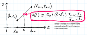
- Linear Interpolation. When the Euler method is used to numerically solve a differential equation what is actually produced is a finite set of discrete points $(t_j, x_j)$ called Euler points. We convert the Euler points into a continuous function using Linear Interpolation. Basically, we connect the Euler points with straight line segments. See image below.
- We actually use a modification of the classical GDA.
What we use is an example of an adaptive GDA. We adapt the learning rate $\eta$ to the size of the gradient. If the length of the gradient vector $ng > 1$ we replace $\eta$ with $\eta/ng$. This has the effect of insuring that the distance between GDA points is at most $\eta$. Note. $ng$ stands for “norm of the gradient” which is a fancy way to say the length of the gradient vector.
Note. The GDA method is based on the fact that the negative of the gradient points in the direction of fast descent. However, this is a local property. We don’t know for how far we can go in that direction (in the direction of the negative of the gradient) and still be descending. If we move too far in that direction, instead of descending, we might be ascending. This is like if you jump over a hole and instead of descending into it, you end up on higher ground. The entire purpose of the GDA is to go down into the hole (to reach a local minimum).

This entry is licensed under a Creative Commons Attribution-NonCommercial-ShareAlike 4.0 International license.