Quiz 2 Type Questions
with Video Solutions
and Maple Scripts
Question 1. Green’s Theorem
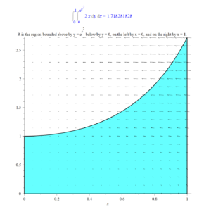
Let $R$ be the region in the x,y plane bounded above by $y = e^{x^2}$, below by $y = 0$, on the left by $x = 0$, and on the right by $x = 1$. See figure below.
Let $c$ be the path about the perimeter of $R$ orientated as indicated by the arrows.
We define the vector field $F(x,y) = \left\langle -xy, \dfrac{x^2}{2}\right\rangle$ on the x,y plane.
Find $\displaystyle{\oint_c F \cdot dr}$ using Green’s Theorem.
Your answer should be accurate to at least the nearest thousandth (3 decimal places).

Solution to Question 1.
Video (6 minutes 45 seconds) on how to solve Question 1.
The following Maple script solves Question 1 using Green’s Theorem:
 restart;
with(plots):
y0 := x -> 0:
y1 := x -> exp(x^2):
x0 := 0:
x1 := 1:
P := (x, y) -> -y*x:
Q := (x, y) -> 1/2*x^2:
# --- no user input needed below this line
miny := minimize(y0(x), x = x0 .. x1):
maxy := maximize(y1(x), x = x0 .. x1):
GI := int(int(diff(Q(x, y), x) - diff(P(x, y), y), y = y0(x) .. y1(x)), x = x0 .. x1):
Int(Int(diff(Q(x, y), x) - diff(P(x, y), y), y = y0(x) .. y1(x)), x = x0 .. x1) = evalf(GI);
mainRegion := shadebetween(y0(x), y1(x), x = x0 .. x1, color = "black", thickness = 3, changefill = [color = "cyan"], title = typeset("R is the region bounded above by y = ", y1(x), " below by y = ", y0(x), ", on the left by x = ", x0, ", and on the right by x = ", x1, "."), size = [1600, 1600]):
a := plot([x0, t, t = y0(x0) .. y1(x0)], color = "black", thickness = 3):
b := plot([x1, t, t = y0(x1) .. y1(x1)], color = "black", thickness = 3):
fp := fieldplot([P, Q], x0 .. x1, miny .. maxy):
display({a, b, mainRegion});
display({a, b, fp, mainRegion});
# End of Maple Script
The above Maple script outputs the solution to Question 1:
Solution to Question 1. The little arrows show the vector field F.
Question 2. Change of Variables Theorem
Find $\iint_S f(x,y) \, dA$ if $f(x,y) = xy$ and $S$ is the parallelogram in the x,y plane having vertices (2,1), (6, 3), (3, 3), and (7, 5). See figure below. Use the change of variables theorem.

Solution to Question 2.
First, a note about the Change of Variables Theorem
The Change of Variables Theorem (in 2 dimensions) tell us that if we can find a differentiable function
$$T:R \rightarrow S$$
bijectively (meaning one-to-one and onto) so that $T(R) = S$,
with
$$T(u,v) = (x(u,v), y(u,v))$$
then
$$\iint_S f(x,y) \, dA = \iint_R f(x(u, v), y(u, v)) \, \left|\dfrac{\partial (x, y)}{\partial (u, v)}\right| \, dA $$
where
$$\dfrac{\partial (x, y)}{\partial (u, v)}$$
is the determinant of the Jacobian matrix:
$$
\begin{pmatrix}
\dfrac{\partial x}{\partial u} & \dfrac{\partial x}{\partial v} \\
\dfrac{\partial y}{\partial u} & \dfrac{\partial y}{\partial v} \\
\end{pmatrix} $$
and where
$$\left|\dfrac{\partial (x, y)}{\partial (u, v)}\right|$$
is the absolute value of the determinant of the Jacobian matrix.
Note. The Change of Variables Theorem is the same in higher dimensions, except now the Jacobian matrix will be an $n \times n$ matrix (in dimension $n$). For example, in dimension 3, we have:
$$
\dfrac{\partial (x, y, z)}{\partial (u, v, w)} =
\det\begin{pmatrix}
\dfrac{\partial x}{\partial u} & \dfrac{\partial x}{\partial v} & \dfrac{\partial x}{\partial w} \\
\dfrac{\partial y}{\partial u} & \dfrac{\partial y}{\partial v} & \dfrac{\partial y}{\partial w}\\
\dfrac{\partial z}{\partial u} & \dfrac{\partial z}{\partial v} & \dfrac{\partial z}{\partial w}\\
\end{pmatrix} $$
Important Confusing Notation Issues!!!
Notation in mathematics is usually very precise. This is not the case with the Jacobian. For some reason, both the Jacobian matrix and the determinant of the Jacobian matrix are often called the Jacobian — which is confusing. To make matters worse the notation
$$\dfrac{\partial (x, y)}{\partial (u, v)}$$
is used to denote both the Jacobian matrix and its determinant (which, of course, are different things). In other words, sometimes that notation means
$$ \dfrac{\partial (x, y)}{\partial (u, v)} =
\text{det}\begin{pmatrix}
\dfrac{\partial x}{\partial u} & \dfrac{\partial x}{\partial v} \\
\dfrac{\partial y}{\partial u} & \dfrac{\partial y}{\partial v} \\
\end{pmatrix} $$
and other times that notation means
$$ \dfrac{\partial (x, y)}{\partial (u, v)} =
\begin{pmatrix}
\dfrac{\partial x}{\partial u} & \dfrac{\partial x}{\partial v} \\
\dfrac{\partial y}{\partial u} & \dfrac{\partial y}{\partial v} \\
\end{pmatrix} $$
In the video of the solution to Question 2 I use
$$\dfrac{\partial (x, y)}{\partial (u, v)}$$
to mean the determinant of the Jacobian matrix.
Further confusing matters, some authors (not me) write the Jacobian matrix in its transpose form. In other words, for them, the Jacobian matrix is the transpose of the more common form. In other words, for those authors, we have:
$$ \dfrac{\partial (x, y)}{\partial (u, v)} =
\begin{pmatrix}
\dfrac{\partial x}{\partial u} & \dfrac{\partial y}{\partial u} \\
\dfrac{\partial x}{\partial v} & \dfrac{\partial y}{\partial v} \\
\end{pmatrix} $$
Which is just the transpose of the more common definition of the Jacobian matrix:
$$ \dfrac{\partial (x, y)}{\partial (u, v)} =
\begin{pmatrix}
\dfrac{\partial x}{\partial u} & \dfrac{\partial x}{\partial v} \\
\dfrac{\partial y}{\partial u} & \dfrac{\partial y}{\partial v} \\
\end{pmatrix} $$
In the above I’m using $ \dfrac{\partial (x, y)}{\partial (u, v)} $ to denote the Jacobian matrix, rather than the determinant of the Jacobian matrix.
Note about the transpose of a matrix. The transpose of a matrix just switches the rows with the columns, for example:
$$\text{transpose}\begin{pmatrix}
a & b \\
c & d \\
\end{pmatrix} = \begin{pmatrix}
a & c \\
b & d \\
\end{pmatrix} $$
The good news is that if A is square matrix then
$$ \text{det} A = \text{det} \left( \text{transpose} A \right)$$
In practice you can almost always figure out what authors intend by their notation by thinking about what makes sense and by the context.
Now, here is the solution to Question 2.
Video of how to solve Question 2
The following Maple script solves Question 2.
restart;
with(plots):
with(VectorCalculus):
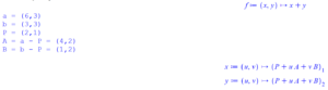
f := (x, y) -> x + y;
P := <2, 1>:
a := <6, 3>:
b := <3, 3>:
# ---- no user input needed below this line ------
A := a - P:
B := b - P:
c := P + A + B:
printf("a = (%a,%a)\n", a[1], a[2]);
printf("b = (%a,%a)\n", b[1], b[2]);
printf("P = (%a,%a)\n", P[1], P[2]);
printf("A = a - P = (%a,%a)\n", A[1], A[2]);
printf("B = b - P = (%a,%a)\n", B[1], B[2]);
x := (u, v) -> (P + u*A + v*B)[1];
y := (u, v) -> (P + u*A + v*B)[2];
uRange := 0 .. 1:
vRange := 0 .. 1:
xmax := max(a[1], b[1], c[1], P[1], 0):
xmin := min(a[1], b[1], c[1], P[1], 0):
ymax := max(a[2], b[2], c[2], P[2], 0):
ymin := min(a[2], b[2], c[2], P[2], 0):
plotRangeX := xmin .. xmax:
plotRangeY := ymin .. ymax:
PA := plot([x(u, 0), y(u, 0), u = uRange], plotRangeX, plotRangeY, scaling = "constrained", color = "red", color = "red", thickness = 5, title = "The region S is the parallelogram shown below", size = [600, 600], labels = ["x", "y"]):
PB := plot([x(0, v), y(0, v), v = vRange], plotRangeX, plotRangeY, scaling = "constrained", color = "blue", thickness = 5):
ac := plot([x(1, v), y(1, v), v = vRange], plotRangeX, plotRangeY, scaling = "constrained", color = "cyan", thickness = 5):
bc := plot([x(u, 1), y(u, 1), u = uRange], plotRangeX, plotRangeY, scaling = "constrained", color = "green", thickness = 5):
tP := textplot([P[1], P[2], typeset("(", P[1], ", ", P[2], ")")], 'align' = {'below', 'right'}):
ta := textplot([a[1], a[2], typeset("(", a[1], ", ", a[2], ")")], 'align' = {'below', 'right'}):
tb := textplot([b[1], b[2], typeset("(", b[1], ", ", b[2], ")")], 'align' = {'above', 'left'}):
tc := textplot([ c[ 1 ] , c[2], typeset("(", c[1], ", ", c[2], ")")], 'align' = {'above', 'left'}):
display({PA, PB, ac, bc, tP, ta, tb, tc});
PAuv := plot([u, 0, u = uRange], uRange, vRange, scaling = "constrained", color = "red", color = "red", thickness = 5, title = "The region R is the square shown below", size = [600, 600], labels = ["u", "v"]):
PBuv := plot([0, v, v = vRange], uRange, vRange, scaling = "constrained", color = "blue", thickness = 5):
acuv := plot([1, v, v = vRange], uRange, vRange, scaling = "constrained", color = "cyan", thickness = 5):
bcuv := plot([u, 1, u = uRange], uRange, vRange, scaling = "constrained", color = "green", thickness = 5):
display({PAuv, PBuv, acuv, bcuv});
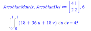
JacobianMatrix, JacobianDet := Jacobian([x(u, v), y(u, v)], [u, v], determinant = true);
Int(Int(f(x(u, v), y(u, v))*abs(JacobianDet), u = uRange), v = vRange) = int(int(f(x(u, v), y(u, v))*abs(JacobianDet), u = uRange), v = vRange);
# End of Script
The above Maple script solves Question 2 and produces the following output:
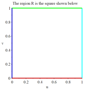
Note 1. $T$ maps the square $R$ to the parallelogram $S$. The red side of the square goes to the red side of the parallelogram, the blue side to the blue side, etc.
Note 2. There is nothing special about the three vertices $(6, 3), (2, 1)$, and $(3, 3)$ that we used to define $a, P$, and $b$, which in turn were used to define $T$. Any three vertices of the parallelogram would have worked provided that the vertex we designate as $P$ is connected to both $a$ and $b$ by an edge 1.
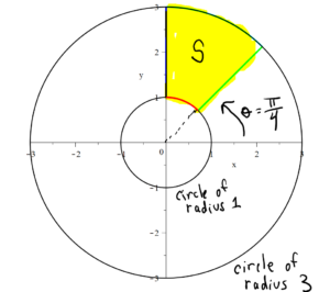
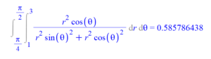
Question 3. Integration using Polar Coordinates
Find
$$\iint_S f(x,y) \, dA$$
if
$$f(x,y) = \dfrac{x}{x^2+ y^2}$$
The region S is the region between the circles of radius 1 and radius 3. S is bounded on the left by the y axis and on the right by the line $y = x$. The line $y = x$ makes an angle of $\dfrac{\pi}{4}$ with the x axis. The region S is shaded yellow in the figure below.
Use polar coordinates.
Solution to Question 3.
Video (less than 5 minutes) showing how to solve Question 3.
The following Maple script solves Question 3.
 restart;
with(plots):
f := (x, y) -> x/(y^2 + x^2);
x := (r, theta) -> r*cos(theta);
y := (r, theta) -> r*sin(theta);
r0 := 1;
r1 := 3;
theta0 := Pi/4;
theta1 := Pi/2;
# ---------------- No user input needed below this line -----
rRange := r0 .. r1:
thetaRange := theta0 .. theta1:
plotRangeR := 0 .. r1:
plotRangeTheta := 0 .. 2*Pi:
plotRange := -r1 .. r1:
aC := plot([r0, theta, theta = thetaRange], plotRangeR, plotRangeTheta, scaling = "constrained", color = "red", color = "red", thickness = 5, labels = ["r", "θ"]):
bC := plot([r, theta1, r = rRange], plotRangeR, plotRangeTheta, scaling = "constrained", color = "blue", thickness = 5):
cC := plot([r1, theta, theta = thetaRange], plotRangeR, plotRangeTheta, scaling = "constrained", color = "cyan", thickness = 5):
dC := plot([r, theta0, r = rRange], plotRangeR, plotRangeTheta, scaling = "constrained", color = "green", thickness = 5):
display({aC, bC, cC, dC});
aa := plot([r0*cos(theta), r0*sin(theta), theta = 0 .. 2*Pi], plotRange, plotRange, scaling = "constrained", color = "black", thickness = 3, labels = ["x", "y"]):
a := plot([r0*cos(theta), r0*sin(theta), theta = thetaRange], plotRange, plotRange, scaling = "constrained", color = "red", color = "red", thickness = 12, labels = ["x", "y"]):
b := plot([r*cos(theta1), r*sin(theta1), r = rRange], plotRange, plotRange, scaling = "constrained", color = "blue", thickness = 12):
cc := plot([r1*cos(theta), r1*sin(theta), theta = 0 .. 2*Pi], plotRange, plotRange, scaling = "constrained", color = black, thickness = 3):
c := plot([r1*cos(theta), r1*sin(theta), theta = thetaRange], plotRange, plotRange, scaling = "constrained", color = "cyan", thickness = 12):
d := plot([r*cos(theta0), r*sin(theta0), r = rRange], plotRange, plotRange, scaling = "constrained", color = "green", thickness = 12):
display({a, aa, b, c, cc, d});
a := plot([r0*cos(theta), r0*sin(theta), theta = thetaRange], plotRange, plotRange, scaling = "constrained", color = "red", thickness = 5, labels = ["x", "y"]):
b := plot([r*cos(theta1), r*sin(theta1), r = rRange], plotRange, plotRange, scaling = "constrained", color = "blue", thickness = 5):
c := plot([r1*cos(theta), r1*sin(theta), theta = thetaRange], plotRange, plotRange, scaling = "constrained", color = "cyan", thickness = 5):
d := plot([r*cos(theta0), r*sin(theta0), r = rRange], plotRange, plotRange, scaling = "constrained", color = "green", thickness = 5):
display({a, b, c, d});
Int(Int(f(x(r, theta), y(r, theta))*r, r = rRange), theta = thetaRange) = int(int(f(x(r, theta), y(r, theta))*r, r = rRange), theta = thetaRange):
Int(Int(f(x(r, theta), y(r, theta))*r, r = rRange), theta = thetaRange) = evalf(int(int(f(x(r, theta), y(r, theta))*r, r = rRange), theta = thetaRange));
# End of Maple Script
The above Maple script solves Question 3 and produces the following output:
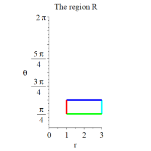
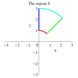
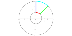
Note. $x = r\, \cos(\theta), \ y = r\, \sin(\theta)$ maps the rectangular region $R = [1, 3] \times \left[\frac{\pi}{4}, \ \frac{\pi}{2} \right]$ to the annular sector $S$. The red edge of R goes to the red edge of $S$, the blue edge to the blue edge, etc.
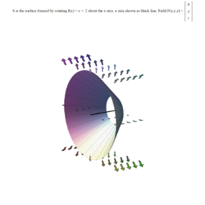
Question 4. Flux Integrals (surface integral of a vector field)
Let $S$ be the surface of revolution formed by rotating $y = x+2$ with $x \in [-1, 1]$ about or around the x-axis. Find the total outward flux passing through $S$ if the vector field $F$ is $F(x,y,z) = \langle 0, y, z \rangle$. For surfaces of revolution “outward” means pointing away from axis of revolution.
Shown below is $S$, the x-axis, and the vector field $F$.
Solution to Question 4.
Video (21 minutes total run time) showing how to solve Question 4
Note about small error in the following video. There is a small error which first appears in Part 1 of the video at 05:56. The screen capture below shows the error, which is that I wrote $(u+2)^2$ when I should have written $(u+2)$.
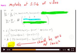
In particular the surface normal vector should be:
$$\dfrac{\partial r}{\partial u} \times \dfrac{\partial r}{\partial v} = \langle (u+2) , – (u+2) \cos(v), -(u+2)\sin(v)\rangle$$
Then, later, at about 09:30 in the same video, this error propagates, and I erroneously put
$$\dfrac{\partial r}{\partial u} \times \dfrac{\partial r}{\partial v}(0,0) = \langle 4 , – 2, 0 \rangle$$
when I should have written:
$$\dfrac{\partial r}{\partial u} \times \dfrac{\partial r}{\partial v}(0,0) = \langle 2 , – 2, 0 \rangle$$
The screen capture below shows this error:

This 2nd error doesn’t effect the orientation of $\dfrac{\partial r}{\partial u} \times \dfrac{\partial r}{\partial v} $ with respect to whether $\dfrac{\partial r}{\partial u} \times \dfrac{\partial r}{\partial v} $ points outward as both $(u+2)^2$ and $u+2$ are positive when $u \in [-1, 1]$.
These errors don’t effect the numerical value of the final answer as the erroneous $(u+2)^2$ term happened to get multiplied by zero in the dot product in the integral and, as mentioned before, the orientation (pointing inward or outward) isn’t effected by this error.
Part 1
Part 2
The following Maple script solves Question 4.
restart;
with(LinearAlgebra):
with(plots):
# ------- Axis of revolution and function f(x) to rotate -----
AxisOfRevolutionString := "x":
AxisOfRevolutionFunction := t -> [t, 0, 0]:
print(cat("Function to be rotated about ", AxisOfRevolutionString, " axis to create the surface S"));
f := x -> x + 2;
# ------------------------- Parametric representation of S ---
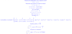
print("Parametric representation of S");
x := (u, v) -> u;
y := (u, v) -> f(u)*cos(v);
z := (u, v) -> f(u)*sin(v);
uStart := -1:
uEnd := 1:
uRange := uStart .. uEnd:
vRange := 0 .. 2*Pi:
r := (u, v) -> <x(u, v), y(u, v), z(u, v)>:
# -------------------------- Vector Field F ----
F1 := (x, y, z) -> 0:
F2 := (x, y, z) -> y:
F3 := (x, y, z) -> z:
F := (x, y, z) -> <F1(x, y, z), F2(x, y, z), F3(x, y, z)>:
# -------------------- No user input needed below this line --
xmin := minimize(x(u, v), u = uRange, v = vRange):
xmax := maximize(x(u, v), u = uRange, v = vRange):
ymin := minimize(y(u, v), u = uRange, v = vRange):
ymax := maximize(y(u, v), u = uRange, v = vRange):
zmin := minimize(z(u, v), u = uRange, v = vRange):
zmax := maximize(z(u, v), u = uRange, v = vRange):
# ----------- Cross product calculation of normal vector N ------
ru := diff(r(u, v), u):
rv := diff(r(u, v), v):
print("Normal to surface"):
ru_X_rv := CrossProduct(ru, rv);
# ---------------------- Needed to plot normal vector ------
uMiddle := (uStart + uEnd)/2:
Nstart := r(uMiddle, 0):
Nend := subs({u = uMiddle, v = 0}, ru_X_rv):
# ----------------------- Integrand calculation -----------
print("Integrand");
F_dot_ru_X_rv := DotProduct(F(x(u, v), y(u, v), z(u, v)), ru_X_rv, conjugate = false);
# ----------------- Flux calculation --------------------------
flux_direct := int(int(F_dot_ru_X_rv, u = uRange), v = vRange):
print("Answer below (may have to be multiplied by -1 depending on orientation)");
Int(Int(F_dot_ru_X_rv, u = uRange), v = vRange) = evalf(int(int(F_dot_ru_X_rv, u = uRange), v = vRange));
# ------------------ Plotting S with solution ---------------------
SurfacePlot := plot3d([x(u, v), y(u, v), z(u, v)], u = uRange, v = vRange, scaling = constrained, title = typeset("S is surface formed by revolving f(x) = ", f(x), " about the ", AxisOfRevolutionString, " axis. ", AxisOfRevolutionString, " axis shown as black line. Field F(x,y,z) = ", F(x, y, z), "\nFlux through surface in direction of surface normal vector ", r[u]," x ", r[v], " (red arrow) = ", flux_direct,"\n Warning! If orientation of red arrow is wrong, multiply answer by -1"), size = [1400, 1400]):
fieldPlot := fieldplot3d([F1(x, y, z), F2(x, y, z), F3(x, y, z)], x = xmin .. xmax, y = ymin .. ymax, z = zmin .. zmax, arrows = THICK, scaling = constrained, grid = [5, 5, 3]):
AxisPlot := spacecurve(AxisOfRevolutionFunction(t), t = uRange, axes = none, color = black, thickness = 5, numpoints = 100):
Nplot := arrow(Nstart, f(uMiddle)*Nend/Norm(Nend, Euclidean), color = red):
display3d(SurfacePlot, fieldPlot, AxisPlot, Nplot);
# --------------------- Plot S without solution ----------------
SurfacePlot := plot3d([x(u, v), y(u, v), z(u, v)], u = uRange, v = vRange, scaling = constrained, title = typeset("S is the surface formed by rotating f(x) = ", f(x), " about the ", AxisOfRevolutionString, " axis. ", AxisOfRevolutionString, " axis shown as black line. Field F(x,y,z) = ", F(x, y, z)), size = [1400, 1400]):
fieldPlot := fieldplot3d([F1(x, y, z), F2(x, y, z), F3(x, y, z)], x = xmin .. xmax, y = ymin .. ymax, z = zmin .. zmax, arrows = THICK, scaling = constrained, grid = [5, 5, 3]):
AxisPlot := spacecurve(AxisOfRevolutionFunction(t), t = uRange, axes = none, color = black, thickness = 5, numpoints = 100):
display3d(SurfacePlot, fieldPlot, AxisPlot);
# End of Maple Script
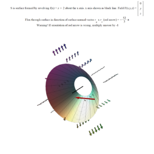
The above Maple script solves Question 4 and generates the following output.

Important note about the above figure and the solution!
Make sure you read this!
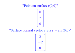
At the point on the surface $r(0, 0) = ( 0, 2, 0)$ the surface normal vector (the little red arrow) is
$$\dfrac{\partial r}{\partial u} \times \dfrac{\partial r}{\partial v} = r_u \times r_v = \langle 2, -2, 0 \rangle$$
Notice that it points inward (towards the x-axis). However, we want the flux in the outward direction to be considered positive. So the orientation of the surface normal vector given by $r_u \times r_v$ is wrong: it should be pointing out of the surface, away from the x-axis. It is easy to fix this. Simply multiply $r_u \times r_v$ by -1.
Or, if you are using Maple to solve the problem, just multiply Maple’s answer by -1.
In particular, the Maple script calculated the flux in the direction of $r_u \times r_v$ and got:
$$-\dfrac{52\pi}{3}$$
however, the correct answer to Question 4 is
$$\dfrac{52\pi}{3}$$
This is because in our parameterization of S, the surface normal vector $r_u \times r_v$ points inward, not outward. So, we have to multiply Maple’s answer by -1 to get the correct answer to Question 4.
Remember. You need to check the orientation of $r_u \times r_v$. If its orientation is wrong, you have to multiply it by -1.
Here is the Maple code to calculate r(0, 0) and $r_u \times r_v$ at $r(0, 0)$. You can add this code to the bottom of the Maple script we used to solve Question 4.
print("Point on surface r(0,0)");
r(0, 0);
print("Surface normal vector r_u x r_v at r(0,0)");
simplify(subs({u = 0, v = 0}, ru_X_rv));
# End of Maple Script
Here is the output of the above Maple code:
The easiest way to determine if a surface normal vector is pointing in the right direction is to sketch it together with the surface. Either by hand or with the help of Maple.
Note. It is enough to check the orientation of $r_u \times r_v$ at a single point.
Question 5. Divergence Theorem
Let $D$ be the solid of revolution formed by rotating $y = x+2$ with $x \in [-1, 1]$ around the x-axis. We can parameterize $D$ by
$$r(u,v,\rho) = (u, \rho (u+2) \cos(v), \rho (u+2) \sin(v)) = (x, y, z)$$
Find the total outward flux passing through the surface $S$ of $D$ if the vector field $F$ is $F(x,y,z) = \langle 0, xy + z , x \rangle$.
Shown below is $D$, a little bit of the x-axis sticking out of D, and the vector field $F$.
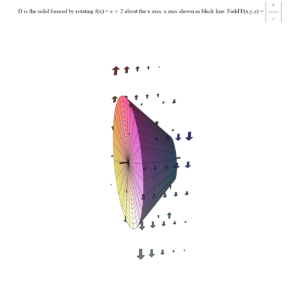
Here is a short video of D being rotated.
Solution to Question 5.
Here is a 16 minute video that shows you how to solve Question 5.
The following Maple Script solves Question 5 using the Divergence Theorem and the Change of Variables Theorem.
restart;
with(LinearAlgebra):
with(plots):
AxisOfRevolutionString := "x":
AxisOfRevolutionFunction := t -> [t, 0, 0]:
print(cat("Function to be rotated about ", AxisOfRevolutionString, " axis to create the solid D"));
f := x -> x + 2;
print("Parametric representation of D solid of revolution");
x := (u, v, p) -> u;
y := (u, v, p) -> p*f(u)*cos(v);
z := (u, v, p) -> p*f(u)*sin(v);
uStart := -1:
uEnd := 1:
uRange := uStart .. uEnd:
LengthOfuRange := uEnd - uStart:
axisOfRotationRange := uStart - LengthOfuRange/5 .. uEnd + LengthOfuRange/5:
vRange := 0 .. 2*Pi:
pRange := 0 .. 1:
r := (u, v, p) -> <x(u, v, p), y(u, v, p), z(u, v, p)>:
print("The vector field F");
F1 := (x, y, z) -> 0;
F2 := (x, y, z) -> y*x + z;
F3 := (x, y, z) -> x;
F := (x, y, z) -> <F1(x, y, z), F2(x, y, z), F3(x, y, z)>:
# ---- No user input needed below this line -------------
"Divergence of F = ";
diff(F1(x, y, z), x) + diff(F2(x, y, z), y) + diff(F3(x, y, z), z);
with(VectorCalculus):
JacobianMatrix, JacobianDet := Jacobian([x(u, v, p), y(u, v, p), z(u, v, p)], [u, v, p], determinant = true);
divF := D[1](F1) + D[2](F2) + D[3](F3):
TotalOutwardFlux := int(int(int(divF(x(u, v, p), y(u, v, p), z(u, v, p))*abs(JacobianDet), u = uRange), v = vRange), p = pRange);
Int(Int(Int(divF(x(u, v, p), y(u, v, p), z(u, v, p))*abs(simplify(JacobianDet)), u = uRange), v = vRange), p = pRange) = TotalOutwardFlux;
xmin := minimize(x(u, v, p), u = uRange, v = vRange, p = pRange):
xmax := maximize(x(u, v, p), u = uRange, v = vRange, p = pRange):
ymin := minimize(y(u, v, p), u = uRange, v = vRange, p = pRange):
ymax := maximize(y(u, v, p), u = uRange, v = vRange, p = pRange):
zmin := minimize(z(u, v, p), u = uRange, v = vRange, p = pRange):
zmax := maximize(z(u, v, p), u = uRange, v = vRange, p = pRange):
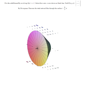
SurfacePlot := plot3d([x(u, v, 1), y(u, v, 1), z(u, v, 1)], u = uRange, v = vRange, scaling = constrained, title = typeset("D is the solid formed by revolving f(x) = ", f(x), " about the ", AxisOfRevolutionString, " axis. ", AxisOfRevolutionString, " axis shown as black line. Field F(x,y,z) = ", F(x, y, z), "\nBy Divergence Theorem the total outward flux through the surface = ", TotalOutwardFlux), size = [1400, 1400]):
print("The answer as a decimal is");
Int(Int(Int(divF(x(u, v, p), y(u, v, p), z(u, v, p))*abs(simplify(JacobianDet)), u = uRange), v = vRange), p = pRange) = evalf(TotalOutwardFlux);
SurfacePlotx0 := plot3d([x(uStart, v, p), y(uStart, v, p), z(uStart, v, p)], v = vRange, p = pRange, scaling = constrained, size = [1400, 1400]):
SurfacePlotx1 := plot3d([x(uEnd, v, p), y(uEnd, v, p), z(uEnd, v, p)], v = vRange, p = pRange, scaling = constrained, size = [1400, 1400]):
fieldPlot := fieldplot3d([F1(x, y, z), F2(x, y, z), F3(x, y, z)], x = xmin .. xmax, y = ymin .. ymax, z = zmin .. zmax, arrows = THICK, scaling = constrained, grid = [5, 5, 3]):
AxisPlot := spacecurve(AxisOfRevolutionFunction(t), t = axisOfRotationRange, axes = none, color = black, thickness = 5, numpoints = 100):
display3d(SurfacePlot, fieldPlot, AxisPlot, SurfacePlotx0, SurfacePlotx1);
SurfacePlot := plot3d([x(u, v, 1), y(u, v, 1), z(u, v, 1)], u = uRange, v = vRange, scaling = constrained, title = typeset("D is the solid formed by rotating f(x) = ", f(x), " about the ", AxisOfRevolutionString, " axis. ", AxisOfRevolutionString, " axis shown as black line. Field F(x,y,z) = ", F(x, y, z)), size = [1400, 1400]):
fieldPlot := fieldplot3d([F1(x, y, z), F2(x, y, z), F3(x, y, z)], x = xmin .. xmax, y = ymin .. ymax, z = zmin .. zmax, arrows = THICK, scaling = constrained, grid = [5, 5, 3]):
AxisPlot := spacecurve(AxisOfRevolutionFunction(t), t = axisOfRotationRange, axes = none, color = black, thickness = 5, numpoints = 100):
display3d(SurfacePlot, fieldPlot, AxisPlot, SurfacePlotx0, SurfacePlotx1);
# End of Maple script
The above Maple script solves Question 5 and produces the following output.
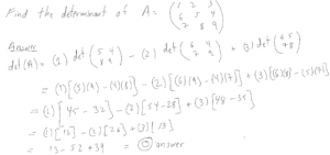
Question 6. Determinants
If
$$
A =
\begin{pmatrix}
1 & 2 & 3 \\
6 & 5 &4 \\
7 & 8 & 9 \\
\end{pmatrix} $$
Find the determinant of $A$.
Solution to Question 6. $\det(A) = 0$ because:
with(LinearAlgebra):
M := Matrix([[1, 2, 3], [6, 5, 4], [7, 8, 9]]);
Determinant(M);
Maple outputs the answer:

Footnotes
- It turns out that there are $4 \times 2 = 8$ affine maps $T$ from the square $R$ to the parallelogram $S$. Four of them preserve orientation “the rotations” and 4 of them are orientation reversing “the reflections” (Jacobian determinant negative). If we let $S = R$ so $T$ is mapping the square to itself, the 8 affine maps of the square to itself form what is called the dihedral group $D_4$. In this case, the affine maps are isometries (meaning they don’t distort distances).

This entry is licensed under a Creative Commons Attribution-NonCommercial-ShareAlike 4.0 International license.