Laplace Transform Videos

Question 1

Solve the above IVP using Laplace Transforms and then find

Answer to Question 1:

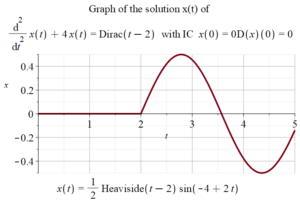
See graph and video below (in 2 parts) for solution. Total run time about 10 minutes.
Part 2 has the final answer.

Part 1.

Part 2.

Notes.
The Heaviside function is the unit step function u(t).
The Dirac function is .

Below are the Maple commands to solve the IVP in Question 1 and create the above Figure. You can copy and paste these commands into Maple.

 de := diff(x(t), t $ 2) + 4*x(t) = Dirac(t - 2);
tq := 2.5;
dsolve(de, x(t));
ics := x(0) = 0, D(x)(0) = 0;
SolutionIVP := dsolve({de, ics});
x(tq) = evalf(subs(t = tq, rhs(SolutionIVP)));
plot(rhs(SolutionIVP), t = 0 .. 5, x = -0.5 .. 0.5, thickness = 4,
  size = [0.5, 0.6], gridlines, 
  title = typeset("Graph of the solution x(t) of \n", de, " with IC ", ics), 
  caption = typeset(SolutionIVP));

Below is a screen capture of above commands in Maple.

Question 2

Solve the above IVP using Laplace Transforms and then find

Answer to Question 2:

See video below (in 5 parts) for solution. Total run time about 30 minutes. Part 5 has the final answer and shows how to solve this question using Maple.

Part 1.