Question 1

,  

Using the Euler method with time step   approximate .

Answer to Question 1:   

  .

See video below (in 2 parts) for the solution. Also, please note the comments, Figure, and Maple code under the last video.  Total run time of the video is about 16 minutes.

Part 1.

 

 

Part 2.

 

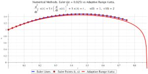
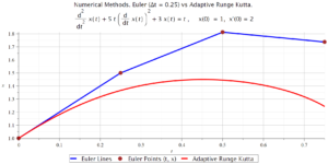
The following two Figures are discussed in Part 2 of the video at about the 4:36 mark.

In these Figures we see graphs of  , from Question 1, approximated by Maple’s built in numerical ODE solver, which uses an Adaptive Runge Kutta method, over the interval ;  and by the Euler method, with , over the interval

The following Figure is the same, except in the Euler method was used. The smaller time step leads to greater accuracy, but is 10 times more computationally intensive.

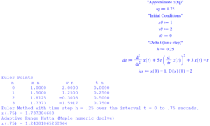
The following Maple commands implement the Euler method for Question 1 and produces the first graph shown above, for the bottom graph change h to 0.025. You can copy and paste the following commands into Maple.

restart;
with(plots):
"Approximate x(tq)";
tq := 0.75;
"Initial Conditions";
x0 := 1;
v0 := 2;
t0 := 0;
tf := tq:
"Delta t (time step)";
h := 0.25;
de := diff(x(t), t $ 2) + 5*t*diff(x(t), t)^2 + 3*x(t) = t;
ics := x(0) = x0, D(x)(0) = v0;
SolutionIVP := dsolve({de, ics}, type = numeric, range = 0 .. 0.87875):
NumOfSteps := (tf - t0)/h:
xn := x0:
vn := v0:
tn := t0:
xnList := [x0]:
tnList := [t0]:
printf("Euler Points\n");
printf("\tn \t    x_n  \t  \t  v_n \t \t  t_n \n");
printf("%5d   %9.4f   %9.4f   %9.4f  \n", 0, xn, vn, tn);
for k to NumOfSteps do
    xnplus1 := h*vn + xn;
    vnplus1 := vn + (-5*tn*vn^2 + tn - 3*xn)*h;
    tnplus1 := tn + h;
    xn := xnplus1;
    vn := vnplus1;
    tn := tnplus1;
    xnList := [op(xnList), xn];
    tnList := [op(tnList), tn];
    printf("%5d   %9.4f   %9.4f   %9.4f  \n", k, xn, vn, tn);
end do:
printf("Euler Method with time step h = %a over the interval t = %a to %a seconds. \n", h, t0, tf);
printf("x(%a) = %a \n", tf, xn);
printf("Adaptive Runge Kutta (Maple numeric dsolve) \n");
printf("x(%a) = %a \n", tf, rhs(op(SolutionIVP(tq))[2]));
ODEplot := odeplot(SolutionIVP, thickness = 6, size = [0.7, 0.5],
 gridlines, color = "red", 
 title = typeset("Numerical Methods. Euler (Δt = ", h, ") vs Adaptive Runge Kutta. \n", de, " ,     x(0)  = ", x0, ",  x'(0) = ", v0), 
 legend = [typeset("  Adaptive Runge Kutta  ")], 
 legendstyle = [font = ["HELVETICA", 24], location = bottom],
 titlefont = ["HELVETICA", 24]):
EulerPlot := plot(tnList, xnList, style = line, thickness = 6,
  color = "blue", legend = [typeset("  Euler Lines  ")], legendstyle = [font = ["HELVETICA", 24], location = bottom]):
EulerPlotPt := plot(tnList, xnList, style = point,
  symbolsize = 12, symbol = solidcircle, color = brown, 
  legend = [typeset("  Euler Points (t, x)  ")], 
  legendstyle = [font = ["HELVETICA", 24], location = bottom]):
display({ODEplot, EulerPlot, EulerPlotPt});

 

---

---

The following Maple script is almost identical to the above. It applies the Euler method to the IVP from Question 1. However, the Runge-Kutta method is implemented over the same interval as the Euler method. As a result, it is suggested that you apply the following Maple script to the differential equations you want to solve using Euler’s method.  Note. If Maple’s implementation of Runge-Kutta “blows up” you will get a warning message as part of the output.

restart;
with(plots):
"Approximate x(tq)";
tq := 0.75;
"Initial Conditions";
x0 := 1;
v0 := 2;
t0 := 0;
tf := tq:
"Delta t (time step)";
h := 0.25;
de := diff(x(t), t $ 2) + 5*t*diff(x(t), t)^2 + 3*x(t) = t;
ics := x(0) = x0, D(x)(0) = v0;
SolutionIVP := dsolve({de, ics}, type = numeric, range = 0 .. tq):
NumOfSteps := (tf - t0)/h:
xn := x0:
vn := v0:
tn := t0:
xnList := [x0]:
tnList := [t0]:
printf("Euler Points\n");
printf("\tn \t    x_n  \t  \t  v_n \t \t  t_n \n");
printf("%5d   %9.4f   %9.4f   %9.4f  \n", 0, xn, vn, tn);
for k to NumOfSteps do
    xnplus1 := h*vn + xn;
    vnplus1 := vn + (-5*tn*vn^2 + tn - 3*xn)*h;
    tnplus1 := tn + h;
    xn := xnplus1;
    vn := vnplus1;
    tn := tnplus1;
    xnList := [op(xnList), xn];
    tnList := [op(tnList), tn];
    printf("%5d   %9.4f   %9.4f   %9.4f  \n", k, xn, vn, tn);
end do:
printf("Euler Method with time step h = %a over the interval t = %a to %a seconds. \n", h, t0, tf);
printf("x(%a) = %a \n", tf, xn);
printf("Adaptive Runge Kutta (Maple numeric dsolve) \n");
printf("x(%a) = %a \n", tf, rhs(op(SolutionIVP(tq))[2]));
ODEplot := odeplot(SolutionIVP, thickness = 6, size = [0.7, 0.5],
 gridlines, color = "red", 
 title = typeset("Numerical Methods. Euler (Δt = ", h, ") vs Adaptive Runge Kutta. \n", de, " ,     x(0)  = ", x0, ",  x'(0) = ", v0), 
 legend = [typeset("  Adaptive Runge Kutta  ")], 
 legendstyle = [font = ["HELVETICA", 24], location = bottom],
 titlefont = ["HELVETICA", 24]):
EulerPlot := plot(tnList, xnList, style = line, thickness = 6,
  color = "blue", legend = [typeset("  Euler Lines  ")], legendstyle = [font = ["HELVETICA", 24], location = bottom]):
EulerPlotPt := plot(tnList, xnList, style = point,
  symbolsize = 12, symbol = solidcircle, color = brown, 
  legend = [typeset("  Euler Points (t, x)  ")], 
  legendstyle = [font = ["HELVETICA", 24], location = bottom]):
display({ODEplot, EulerPlot, EulerPlotPt});

The above Maple script outputs the following.

 

---

Here is a much simpler Maple script to calculate the Euler Points for Question 1. It uses Maple’s built in Euler numerical method. It doesn’t produce a graph though.

restart;
ode := diff(x(t), t $ 2) + 5*t*diff(x(t), t)^2 + 3*x(t) = t;
ics := x(0) = 1, D(x)(0) = 2;
t_initial := 0;
t_final := 0.75;
delta_t := 0.25;
############################################ 
#### End of user input #####################
############################################
t0 := t_initial:
tf := t_final:
numSteps := ceil((t_final - t_initial)/delta_t);
interface(rtablesize = numSteps + 1):
EulerSolution := dsolve({ics, ode}, numeric, method = classical[foreuler], stepsize = (tf - t0)/numSteps, output = Array([seq(t0 .. tf, (tf - t0)/numSteps)])):
EulerSolution[1, 1];
EulerPoints := EulerSolution[2, 1];
ans := EulerPoints[numSteps + 1, 2]:
printf("Euler Method with time step delta_t = %a over the interval t = %a to %a seconds. \n", delta_t, t0, tf);
printf("x(%a) = %a (Euler approximation) \n", tf, ans); 
# End of Maple Script

Here is the output of the above Maple script:

Here is Python 3 code which will implement the Euler Method for Question 1 above. It doesn’t produce a graph though. However, it might be simpler to read than the Maple code.

You can run the following Python 3 code online, for free, at:
https://trinket.io/features/python3

# Written by Chris McCarthy Oct 2022
#=========================================== for online compilers
import matplotlib as mpl
mpl.use('Agg')
#=========================================== usual packages
import numpy as np
from matplotlib import pyplot as plt
plt.rcParams.update({'font.size': 22})
#============================================
# Example
#==============================
# ODE x'' + 5t(x')^2 + 3x = t 
# IC x(0) = 1, xdot(0)=2
# Approximate x(0.75) using the Euler method with Delta t = 0.25
#
# Solution: T(x,v,t) =
# xdot = v
# vdot = -5*t*v^2 - 3*x + t
# tdot = 1
#
# USER INPUT STARTS HERE
# =========================
def vdot(x,v,t):
    return -5*t*v**2 - 3*x + t
# 0th Euler Point (IC)
x0=1
v0=2
t0=0
#
Delta_t = 0.25
#
# final time
tf = .75
#
# USER INPUT ENDS HERE
# =========================
def T(xvt): #tangent vector (input np.array object xvt)
    x = xvt[0]
    v = xvt[1]
    t = xvt[2]
    return np.array([v, vdot(x,v,t) , 1 ])
def EulerStep(T, xvt, Delta_t):
    return xvt + Delta_t*T(xvt) 
#
N = int( (tf-t0)/Delta_t ) # Number of steps
xvt = np.array([x0, v0, t0]) # define first Euler point
print(' ')
print('The Euler Points')
print(xvt) 
#
for n in range(N): # Euler recursion
    xvt = EulerStep(T, xvt, Delta_t)
    print(xvt)
#
#============================================= 
print(' ')
print('The Euler Method approximation of x(', xvt[2], ') is ', xvt[0])
print(' ')
print('The Euler Method approximation of xdot(', xvt[2], ') is ', xvt[1])
#=============================================
# End of code

 

Notes about using the above Python code

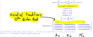
You can copy and paste the above code into an online Python 3 compiler or into your Python 3 editor on your own computer. The only part of the above code you need to modify (if you want to use this code for a different differential equation) is the part indicated in the picture below.

If you want to use this code for a different differential equation, you need to tell Python what $\dot{v}$ is vdot, what the $0^{th}$ Euler Point is, x0, v0, t0; what $\Delta t$ is Delta_t, and what the the time is that you want $x(t)$ approximated at tf.

With Python you need to be very careful about indents. Make sure you don’t change the number of spaces in the indented parts. If you do, you will get an error message.

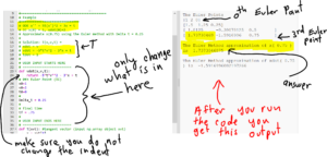
The above picture is a screen grab of the Python 3 code using Euler’s Method to solve Question 1, showing the part of the code that needs to be changed if you change the differential equation.

Question 2 (no video available for this question)

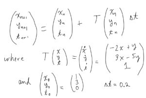
$\dot{x} = -2x + y,  \ \ \ \ x(0) = 1 $
$\dot{y} = 3x – 5y, \ \ \ \ \ \ \ \ y(0) = 3 $
Using the Euler Method with a time step of $\Delta t = 0.2$ estimate x(0.6) and y(0.6).

Answer to Question 2 (using Maple)

 

We iterate

Using Maple to implement the above Euler scheme, we get:

$x(0.6) \approx 0.648$

$y(0.6) \approx 0.504$

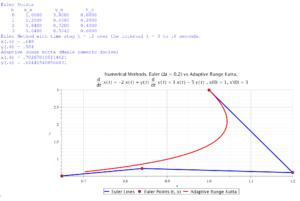
The Maple script to solve Question 2 and produce the above graph is below.  You can copy and paste the script into Maple.

 

restart;
with(plots):
a := -2;
b := 1;
c := 3;
d := -5;
xx := (x, y) -> a*x + b*y;
yy := (x, y) -> c*x + d*y;
x0 := 1:
y0 := 3:
tq := 0.6:
t0 := 0:
tf := tq;
h := 0.2;
dex := diff(x(t), t) = xx(x(t), y(t));
dey := diff(y(t), t) = yy(x(t), y(t));
de := diff(x(t), t) = xx(x(t), y(t)), diff(y(t), t) = yy(x(t), y(t)):
de := dex, dey:
ics := x(0) = x0, y(0) = y0:
ans := dsolve([de, ics]):
SolutionIVP := dsolve({de, ics}, type = numeric, range = 0 .. tq):
ODEplot := odeplot(SolutionIVP, [x(t), y(t)], thickness = 6, size = [0.7, 0.5], gridlines, color = "red", title = typeset("Numerical Methods. Euler (Δt = ", h, ") vs Adaptive Runge Kutta. \n", de, " , x(0) = ", x0, ", x'(0) = ", y0), legend = [typeset(" Adaptive Runge Kutta ")], legendstyle = [font = ["HELVETICA", 24], location = bottom], titlefont = ["HELVETICA", 24]):
NumOfSteps := (tf - t0)/h:
xn := x0:
yn := y0:
tn := t0:
xnList := [x0]:
ynList := [y0]:
tnList := [t0]:
printf("Euler Points\n");
printf("\tn \t x_n \t \t y_n \t \t t_n \n");
printf("%5d %9.4f %9.4f %9.4f \n", 0, xn, yn, tn);
for k to NumOfSteps do
xnplus1 := xn + h*xx(xn, yn):
ynplus1 := yn + h*yy(xn, yn):
tnplus1 := tn + h:
xn := xnplus1:
yn := ynplus1:
tn := tnplus1:
xnList := [op(xnList), xn]:
ynList := [op(ynList), yn]:
tnList := [op(tnList), tn]:
printf("%5d %9.4f %9.4f %9.4f \n", k, xn, yn, tn);
end do:
printf("Euler Method with time step h = %a over the interval t = %a to %a seconds. \n", h, t0, tf);
printf("x(%a) = %a \n", tf, xn);
printf("y(%a) = %a \n", tf, yn);
printf("Adaptive Runge Kutta (Maple numeric dsolve) \n");
printf("x(%a) = %a \n", tf, rhs(op(SolutionIVP(tq))[2]));
printf("y(%a) = %a \n", tf, rhs(op(SolutionIVP(tq))[3]));
EulerPlot := plot(xnList, ynList, style = line, thickness = 6, color = "blue", legend = [typeset(" Euler Lines ")], legendstyle = [font = ["HELVETICA", 24], location = bottom]):
EulerPlotPt := plot(xnList, ynList, style = point, symbolsize = 12, symbol = solidcircle, color = brown, legend = [typeset(" Euler Points (t, x) ")], legendstyle = [font = ["HELVETICA", 24], location = bottom]):
display({ODEplot, EulerPlot, EulerPlotPt});

---