The Gradient Descent Algorithm (GDA) is an algorithm used to find the minimum of a function.

In these notes we will concentrate on minimizing functions of two variables, i.e.,  $f(x, y),$ however the GDA can be applied to functions of more than two variables – or even just a single variable, i.e., $f(x).$

In these notes we will present the basic GDA.  In practice, the basic GDA is often tweaked to help ensure convergence or to speed up convergence.

The Gradient. We write the gradient of a function $f(x, y)$ using the “nabla” symbol $\nabla.$ For example
$$\nabla f = \left\langle \frac{\partial f}{\partial x}, \frac{\partial f}{\partial y} \right\rangle  $$

Here is the GDA

Let $(x_0, y_0)$ be given, then:
$$ (x_{j+1}, y_{j+1}) = (x_j, y_j) \ – \  \eta\  \,  \nabla f(x_j, y_j)$$
Typically, one runs the GDA algorithm until
$$|| (x_{j+1}, y_{j+1}) \ – \  (x_j, y_j)||$$
is sufficiently small, or until
$$|| f(x_{j+1}, y_{j+1}) \ – \  f(x_j, y_j)||$$
is sufficiently small, or for a specified number of iterations.

$\eta$, pronounced “eta” is sometimes called the “learning rate”, especially when the GDA is used in the context of machine learning (AI).

Notation.

$|| (x_{j+1}, y_{j+1}) \ – \ (x_j, y_j)||  = \ \ \ \ \ \ \ $

$ \ \ \ \ \ \ \ \sqrt{(x_{j+1} \ – \ x_j)^2  + (y_{j+1} \ –  \  y_j)^2 } $

which is just the usual Euclidean distance formula from the Pythagorean Theorem.

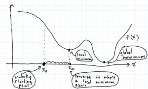
Note.  Don’t forget, if the GDA produces a sequence of points which converge, they may converge to where a local minimum occurs, rather than to where the global minimum occurs. For an example of this, see the picture a few paragraphs down.

Note. The important things to remember are that the starting point $(x_0, y_0)$ of the GDA  and the learning rate $\eta$ both can have an effect on to where and if the GDA points converge.

About the GDA. The GDA is based on the theorem that states that a function $f(x,y)$ decreases most rapidly in the opposite direction of its gradient, meaning in the $-\nabla f$ direction. It is important to understand that if we travel in the $-\nabla f$ that $f$ will initially decrease, however, we don’t know for how long $f$ will keep decreasing.

The GDA produces a sequence of points $(x_j, y_j)$, which, with luck, will converge on a point $(x_m, y_m)$ that minimizes (at least locally) the function $f$. There are various theorems which give conditions under which convergence is guaranteed. However, it is often difficult to check whether these conditions are satisfied. Hence the statement about “with luck”.

The GDA can also be applied to functions of one variable, e.g., to $f(x)$. In the following picture we see an unlucky choice of starting point for the GDA as the GDA points converge to where a local minimum occurs, rather than to where the global minimum occurs. In other words where you start the GDA can have an huge effect on where and if the GDA points converges.

For a video about the GDA and a Maple Script to implement the GDA see:
https://mccarthymat501.commons.gc.cuny.edu/calculus-i-iii/mat-303-calculus-iii/mat-303-quiz-1/

GDA implemented in R.

In the following 16 second video we see the surface
$$z = f(x,y) = \sin\left( \dfrac{x^2 + y^2}{3} \right)$$
together with the GDA points (green) lifted to the surface $z$ by $f$.

Technically speaking, the GDA points are not on the surface $z$. They are the points $(x_n, y_n)$ in the x,y plane that are generated by the GDA.  However, we will call the points $(x_n, y_n, f(x_n, y_n))$ GDA points too, since it is tedious to say “GDA points lifted to the surface $z$ by $f$.

In the R script and in the image below, the GDA starting point is $(x_0, y_0) = (1, 2).$ The green point, which you can see by itself in the first frame of video, is located at  $(x, y, z) = (1, 2, f(1, 2))$, which is at the top of the inner wave. In the video below, you can see the path that the green GDA points take as they descend to a local minimum (red).

 

Here is the R script used to implement the GDA and which output the 3D graph shown in the video.  The following R script requires the package “rgl” to make the 3D graph.

library(rgl) # for 3d plots

# the function to minimize
f <- function(x, y){
 sin( ((x)^2 + (y)^2)/3 ) 
}

# numerical gradient
grad <- function(x,y,f){
 h = 0.001
 fx = ( f(x + h, y) - f(x - h, y) )/ (2*h)
 fy = ( f(x, y + h) - f(x, y - h) )/ (2*h)
 c(fx, fy) 
}

#starting point for GDA
x0 = 1
y0 = 2

# iterations
its = 1000;

#################################
# no user input needed below here
# initialize vectors x and y
x = c(x0)
y = c(y0)

# GDA
for (k in 1:(its - 1) ) {
 eta = 0.01 # learning rate
 x[k+1] = x[k] - eta*grad(x[k], y[k], f)[1]
 y[k+1] = y[k] - eta*grad(x[k], y[k], f)[2]
}

# plots
id = plot3d(f, col = colorRampPalette(c("blue", "white")), 
 xlab = "X", ylab = "Y", zlab = "Z", 
 xlim = c(-5, 5), ylim = c(-5, 5),
 aspect = c(1, 1, 0.5))
 contourLines3d(id) # "z" is the default function
 rgl.spheres(x, y, f(x,y), r = .2, color = "green") 
 rgl.spheres(x[its], y[its], f(x[its], y[its]), r = .4, color =  "red")
# End R script

For information about R, including a brief 3 1/2 minute video tutorial, how to download it for free, and how to run it online for free, see my page:
https://mccarthymat150.commons.gc.cuny.edu/r/