Quiz 1 Type Questions
with Video Solutions
and Maple Scripts

Question 1. Gradient Descent Algorithm (GDA)

Let
$f(x,y) = (x-1)^2 (y-3)^2$
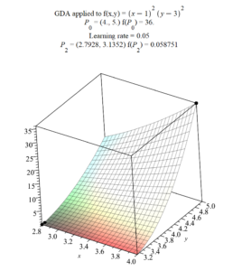
$P_0 = (x_0, y_0) = (4, 5)$
$\eta = 0.05$

Using the gradient descent algorithm find $P_2 = (x_2, y_2)$ and then calculate $f(P_2)$ to at least the nearest thousandth (at least 3 decimal places).

Note. The gradient descent algorithm can be written as
$$P_n = P_{n-1} – \eta \nabla f(P_{n-1})$$

Note. $\eta$ is sometimes called the “learning rate”. Especially in the context of machine learning (AI).

Solution to Question 1.

 

The following Maple script implements the Gradient Descent Algorithm and solves the above Question.

 # Gradient Descent Algorithm GDA
restart;
with(plots):
with(Student[VectorCalculus]):
f := (x, y) -> (x - 1)^2*(y - 3)^2;
starting_point := [4, 5]:
learning_rate := 0.05:
n_to_stop_at := 2:
# ------- No input needed below this line ------------
h := learning_rate:
pointsInPath := (Student[VectorCalculus]):-`+`(n_to_stop_at, 1):
gradf := [diff(f(x, y), x), diff(f(x, y), y)];
printf("learning rate = %3.3f\n", h);
search_radius := 1000000:
pINITIAL := starting_point:
pList := [pINITIAL]:
Pintitial3D := [pINITIAL[1], pINITIAL[2], f(pINITIAL[1], pINITIAL[2])]:
myList := [evalf(Pintitial3D)]:
for i to (Student[VectorCalculus]):-`+`(pointsInPath, -1) do
pOLD := pList[i];
pNEW := (Student[VectorCalculus]):-`+`(pOLD, (Student[VectorCalculus]):-`-`((Student[VectorCalculus]):-`*`(h, subs(x = pOLD[1], y = pOLD[2], gradf))));
pNEW := evalf(pNEW);
pList := [op(pList), pNEW];
if search_radius < (Student[VectorCalculus]):-`+`((Student[VectorCalculus]):-`+`(abs(pNEW[1]), abs(pNEW[2])), abs(evalf(f(pNEW[1], pNEW[2])))) then
print("GDA terminated early. Magnitude of numbers too large. ");
pointsInPath := i;
break;
end if;
end do:
for i from 2 to pointsInPath do
p2d := pList[i];
p3d := [p2d[1], p2d[2], f(p2d[1], p2d[2])];
myList := [op(myList), p3d];
end do:
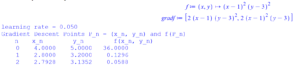
printf("Gradient Descent Points P_n = (x_n, y_n) and f(P_n) \n");
printf("\tn \t x_n \t \t y_n \t \t f(x_n, y_n) \n");
for n to pointsInPath do
P1 := myList[n][1];
P2 := myList[n][2];
printf("%5d %9.4f %9.4f %9.4f \n", (Student[VectorCalculus]):-`+`(n, -1), P1, P2, evalf(f(P1, P2)));
end do:
minx := min(myList[1 .. pointsInPath, 1]):
miny := min(myList[1 .. pointsInPath, 2]):
maxx := max(myList[1 .. pointsInPath, 1]):
maxy := max(myList[1 .. pointsInPath, 2]):
xRange := minx .. maxx:
yRange := miny .. maxy:
P0x := evalf[5](myList[1, 1]):
P0y := evalf[5](myList[1, 2]):
f0 := evalf[5](myList[1, 3]):
Pnx := evalf[5](myList[pointsInPath, 1]):
Pny := evalf[5](myList[pointsInPath, 2]):
fn := evalf[5](myList[pointsInPath, 3]):
a := plot3d(f(x, y), x = xRange, y = yRange, title = typeset("GDA applied to f(x,y) = ", f(x, y), "\n", P[0], " = (", P0x, ", ", P0y, ") f(", P[0], ") = ", f0, "\n Learning rate = ", h, " \n", P[(Student[VectorCalculus]):-`+`(pointsInPath, -1)], " = (", Pnx, ", ", Pny, ") f(", P[(Student[VectorCalculus]):-`+`(pointsInPath, -1)], ") = ", fn), size = [1600, 1000]):
b := pointplot3d(myList, symbol = solidsphere, symbolsize = 15, color = black):
display(a, b);
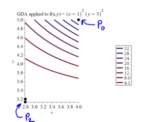
ca := contourplot(f(x, y), x = xRange, y = yRange, thickness = 5, title = typeset("GDA applied to f(x,y) = ", f(x, y)), legend = [digits = 2], legendstyle = [font = [Times, roman, 18], location = right], size = [800, 600]):
cb := pointplot(pList, symbol = solidcircle, symbolsize = 15, color = black, scaling = constrained, axes = normal):
display(ca, cb);
# End Maple GDA Script

Here is the output of the above Maple script (solving Question 1):

 

If, in the Question 1, the learning rate is .005, and we have Maple calculate the GDA points $P_0$ to $P_{200}$, we get the following results.

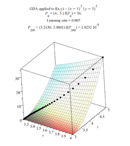
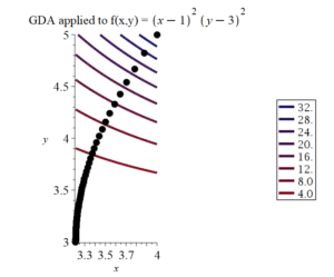
In the above Figure, notice how the GDA path, shown as blue circles, is perpendicular to the contour lines of $f(x,y)$.

Question 2A. Double Integral (Integrate in the x direction first)

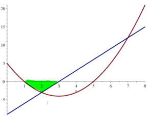
D is the region bounded below (and on the left) by $y = (x-3)^2 – 4$; below (and on the right) by $y = 3x-9$; and above by the x-axis. If $f(x,y) = 72(x-3)y$ find

$$\iint_D f(x,y)\, dA$$.

D is the green region shown below.

Solution to Question 2A.

 

The following Maple script calculates the double integral if we integrate in the $x$ direction first and solves the above Question.

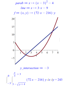
 # Double Integral dx dy
parab := x -> (x - 3)^2 - 4;
line := x -> 3*x - 9;
f := (x, y) -> 72*(x - 3)*y;
plot([parab(x), line(x)], x = 0 .. 8, thickness = 5);
y_intersection := solve(3 - sqrt(y + 4) = (y + 9)/3, y);
Int(Int(f(x, y), x = 3 - sqrt(y + 4) .. (y + 9)/3), y = -3 .. 0) = int(int(f(x, y), x = 3 - sqrt(y + 4) .. (y + 9)/3), y = -3 .. 0);
# End Maple Script

Here is the output of the above Maple script (solving Question 2A):

Question 2B. Double Integral (Integrate in the y direction first)

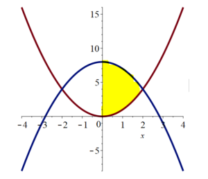
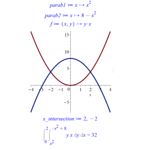
D is the region bounded above by $y = 8 – x^2$; below by $y = x^2$; and on the left by the y-axis. If $f(x,y) = xy$ find

$$\iint_D f(x,y)\, dA$$.

D is the yellow region shown below.

Solution to Question 2B.

We will integrate in the $y$ direction first from $y = x^2$ to $y = 8 – x^2$. Then, we will integrate in the $x$ direction, from $x = 0$ to the x-coordinate of where the two parabolas intersect. To find the x-coordinate of the intersection solve $x^2 = 8 – x^2$ for $x$.  A little algebra gives us $2x^2 = 8$ or $x^2 = 4$. So, $x = \pm 2$. With $x = 2$ being the x-coordinate of the parabola’s intersection point in D. So, the limits of integration for $dx$ are $x = 0$ to $x = 2$.

$ \displaystyle  \iint_D f(x,y) \, dA = \iint_D f(x,y) \, dy\,  dx$
$\displaystyle  =  \int_{x = 0}^{x = 2} \int_{y = 8-x^2}^{y = x^2} xy \, dy\,  dx$
$=  \left.\displaystyle \int_{0}^{2}  \dfrac{xy^2}{2}  \right\rvert^{y = 8-x^2}_{y = x^2}  \,  dx$
$=  \displaystyle \int_{0}^{2}  \dfrac{x\left(8-x^2\right)^2}{2} – \dfrac{x\left(x^2\right)^2}{2}    \,  dx $
$=  \displaystyle \dfrac{1}{2} \, \int_{0}^{2} x\left(64 – 16x^2  + x^4\right) – x\left(x^4\right)    \,  dx $
$=  \displaystyle \dfrac{1}{2} \, \int_{0}^{2} 64x – 16x^3   \,  dx $
$=  \left.\displaystyle   \dfrac{1}{2} \, \left(  \dfrac{64x^2}{2} – \dfrac{16x^4}{4} \right) \right\rvert_{x = 0}^{x = 2}  $
$=  \left.\displaystyle     \dfrac{1}{2} \, \left(32x^2 – 4x^4 \right) \right\rvert_{x = 0}^{x = 2}  $
$=  \displaystyle   \dfrac{1}{2} \, \left(\left(32(2)^2 – 4(2)^4\right) – \left(32(0)^2 – 4(0)^4\right)  \right)$
$=  \displaystyle    32(2)^1 – 4(2)^3 $
$=  64 – 32$
$=  32$ (answer)

The following Maple script calculates the double integral if we integrate in the $y$ direction first and solves the above Question.

 # Double Integral dy dx
parab1 := x -> x^2;
parab2 := x -> 8 - x^2;
f := (x, y) -> y*x;
plot([parab1(x), parab2(x)], x = -4 .. 4, thickness = 5);
x_intersection := solve(parab1(x) = parab2(x), x);
Int(Int(f(x, y), y = parab1(x) .. parab2(x)), x = 0 .. 2) = int(int(f(x, y), y = parab1(x) .. parab2(x)), x = 0 .. 2);
# End Maple Script

Here is the output of the above Maple script (solving Question 2B):

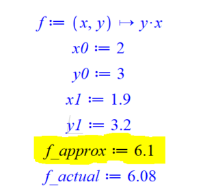
Question 3. Linear approximation.

$f(x,y) = xy$.  Linearly approximate $f(1.9, 3.2)$ using $f(2,3) = 6$.

Solution to Question 3.

 

The following Maple script calculates the linear approximation and solves the above Question.

 # Linearly approximation
f := (x, y) -> x*y;
x0 := 2;
y0 := 3;
x1 := 1.9;
y1 := 3.2;
f_approx := f(x0, y0) + subs([x = x0, y = y0], diff(f(x, y), x))*(x1 - x0) + subs([x = x0, y = y0], diff(f(x, y), y))*(y1 - y0);
f_actual := f(x1, y1);
# End Maple Script

Here is the output of the above Maple script (solving Question 3):

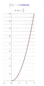
Question 4. Vector Line Integrals (Work Integrals)

Let $F(x,y) = \langle xy, x – y \rangle$ be a vector field on $\mathbb{R}^2$. Let $C$ be the parabolic path from $(0, 0)$ to $(3, 9)$ parameterized as $r(t) = (t, t^2)$ with $t$ going from $0$ to $3$. Find $\int_C F \cdot dr$

Solution to Question 4.

 

The following Maple script calculates the vector line integral (the work integral), plots the trajectory $C$, shows the vector field $F$, and solves the above Question.

 #Vector line integral (work integral)
with(LinearAlgebra):
with(plots):
P := (x, y) -> x*y:
Q := (x, y) -> x - y:
F := (x, y) -> <P(x, y), Q(x, y)>:
x := t -> t:
y := t -> t^2:
c := t -> <x(t), y(t)>:
tRange := 0 .. 3:
vector_line_integral := int(DotProduct(F(x(t), y(t)), diff(c(t), t)), t = tRange):
pc := plot([x(t), y(t), t = tRange], thickness = 4, scaling = constrained, title = typeset("&int; F &middot;dr = ", vector_line_integral)):
fp := fieldplot([P, Q], -1 .. 3, 0 .. 9):
Int(F, r) = evalf(vector_line_integral);
display({fp, pc});
# End Maple Script 

Here is the output of the above Maple script (solving Question 4):