Newton’s Law of Cooling

Newton’s Law of Cooling ¹ is based on the differential equation , where $y(t)$ is the temperature of the body and $T$ is the temperature of the environment surrounding the body.

Scenario: You have hot water (initial temperature $y_0$ ) in a container, say a cup. The temperature in the room is cooler, say a constant $T$ degrees Celsius. Come up with a differential equation which models the water’s temperature $y(t)$ as a function of time $t$ .

Model: The rate at which the water cools should be proportional to how much cooler the room is than the water. For example, if the air temperature is much colder than the water, the water will cool down more quickly than if the air temperature is closer to the water’s temperature. So, $\dfrac{dy}{dt}$ should be proportional to the difference in temperature: $T - y$ , in other words, we should have:

$y' = k(T-y)$ with IC $y(0) = y_0$ ,

where $k > 0$ is the constant of proportionality. This differential equation is easily solved by separation as follows.

$\dfrac{dy}{dt} = k(T-y)$

$\dfrac{dy}{T-y} = k \, dt$

$\displaystyle \int \dfrac{dy}{T-y} = \int k \, dt + c_1$

$-\ln|T-y| = kt + c_1$ ,

which implies

$T - y = c_2 e^{-kt}$ ,

and so we get the general solution:

$y = T + c_3 e^{-kt}$ .

Using the IC, we get

$y_0 = T + c_3$ ,

so,

$c_3 = y_0 - T$

We arrive at Newton’s Law of Cooling:

$y(t) = T + (y_0 - T)e^{-kt}$

Warning: Newton’s Law of Cooling is a beautiful, mathematically simple approximation of what actually happens as bodies cool. One should not expect the same level of accuracy from his law of cooling, as say from Newton’s Law of Gravitation. For a fascinating discussion of the history and accuracy of Newton’s Law of Cooling see ².

Note: Newton’s Law of Cooling will be exactly the same if the water temperature $y$ is colder than the the air temperature $T$ . In other words, Newton’s Law of Cooling also works for heating.

Note: We could measure temperature using Fahrenheit instead of Celsius.

About models. We build mathematical models by using common sense logical reasoning, mathematical intuition, our experiences, physical laws, and hopeful guessing. In the end, a model is just a hopeful guess, and we should test our model with real world data (for example, by doing experiments). See below. For more about the relationship of mathematical models to realty, see ³.

Newton’s Law of Cooling Experiment

(Left) A 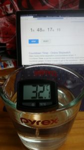photograph of the experiment showing how the
(time $t_i$ , temperature $y_i$ ) measurements were done. In the background is an online stopwatch/timer which gives the elapsed time. In the foreground is 500 mL of hot water in a Pyrex measuring cup. Initially the water temperature was $y_0 = 81.0^{\circ}$ C ( $177.8^{\circ}$ F). The air temperature remained (for the most part) a constant $T = 28.6^{\circ}$ C ( $78^{\circ}$ F). To measure the temperature a Weber 6492 Instant Read Digital Thermometer was used. As the experiment ran, the set up was photographed (cell phone). The time, temperature measurements were recorded manually from the photos. The Weber 6492 is typically used for cooking. It costs about $10 (2018 prices) and is easily available online or at cooking stores and hardware stores. The experiment was conducted Feb 9, 2018. The data and analysis of the experiment are discussed below:

In our experiment, Newton’s Law of Cooling,

$y(t) = T + (y_0 - T)e^{-kt}$

with $y_0 = 81.0^{\circ}$ C and $T = 28.6^{\circ}$ C, becomes:

$y(t) = 28.6 + 52.4 e^{-kt}$

Finding k.
We can use R’s nonlinear regression command “nls” to find the k which will make

$y(t) = T + (y_0 - T)e^{-kt}$

fit the data as closely as possible. The R command “nls” works best if we can supply it with a starting estimate for k. An easy way to estimate k is to solve

$y(t) = T + (y_0 - T)e^{-kt}$

for k:

$k = \dfrac{\ln \left(\dfrac{y_0 - T}{y(t) - T}\right)}{t}$

Then each data point $(t_i, y_i)$ gives an estimate $k_i$ of k:

$k_i = \dfrac{\ln \left(\dfrac{y_0 - T}{y_i - T}\right)}{t_i}$

In the R script below, the estimate of k that we provide to “nls” is the median of the $k_i$ .

Analyzing the data using the open source (free) statistical software R.
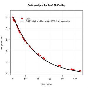
We used R’s nonlinear regression command “nls” to find the value for $k$ which will make $y(t) = 28.6 + 52.4 e^{-kt}$ mostly closely fit the data (the red circles in the graph shown below). The best value for $k$ that R found was $k = 0.026705$ . We then had R plot the data (red circles) together with the “prediction” or “regression curve” ⁴ :

$y(t) = 28.6 + 52.4 e^{- 0.026705t}$

(the black curve). As you can see in the graph below, the curve matches the data fairly closely.

The R script. The following code did the data analysis (discussed in the preceding paragraph) and created the graph shown above. You can copy and paste the following R code into R (running on your own computer) or online at:

rdrr https://rdrr.io/snippets
mycompiler https://www.mycompiler.io/online-r-compiler

and it should run without modification.
Note. The above two R-online sites have been most recently tested March 2022.

Important note! If you use this code with new data make sure you give T and y0 in the same units (F or C) as your data.

#  RcodeNewtonLawOfCoolingRegPlot.R
#  Does regression on data from Newton's Law of Cooling Experiment and
#  plots results. For Mat 501 notes. 

# Experiment notes:    Date: Feb 9, 2018 
# 500 mL of near to boiling water in a pyrex measuring cup.
# about 50 mL evaporated eventually.

# air and initial water temp (C)
T = 28.6  # air temp (78 deg F) 
y0 = 81.0 # initial water temperature (177.8 deg F)

# data from experiment taken manually 
# (t_i, y_i) = (time in min, water temp in C);

# t_i time data (min) Note a measurement like 60+34+9/60 means 1 hr 34 min 9 sec
t_i = c(4/60, 30/60,  1,   1+31/60, 2  ,2+30/60, 3+2/60, 3+34/60,
 6+35/60, 7+17/60,8+30/60, 9+39/60,10+30/60, 11+24/60, 13+11/60, 15 + 37/60, 17+6/60,
 19+23/60,21+43/60, 26+51/60, 26+55/60,31+41/60, 40+44/60,44+6/60, 48+42/60, 50+38/60,
 60+14+12/50, 60+16+10/60, 60+34+9/60, 60+35+20/60, 60+38+4/60, 60+48+17/60 );     

# y_i water temperature data (C) 
y_i =  c(80.0, 78.3,  77.6, 77.6,  77.2 , 76.5 ,  76.3,  76.6,  
 72.6, 71.3, 69.8, 68.2, 67.2, 66.1, 64.3, 62.2, 60.6,
 58.9, 57.1, 54.0, 54.0, 51.3, 47.2, 45.8,43.8, 43.1,
 37.0, 36.6, 33.6, 33.5, 33.1, 32.1);    

# display data in console.
t_i;    
y_i;

# approximate k
"k_estimate";
k_est = median(log((y0-T)/(y_i - T))/t_i, na.rm=TRUE); 
            # na.rm=TRUE fixes t_i = 0 divide by zero issue 
k_est;

# make data frame to hold data
df = data.frame(t_i, y_i );
df;

# Do the non linear regression calculation
regressionCalculation = nls(  y_i ~ (  T + (y0 - T)*exp(-k*t_i) ),  
 data = df,               # use the data stored in df
 start = list(k = k_est), # we guess that k is about k_est
 trace = T);              # gives information about calculation 

# output results of regressionCalculation
summary(regressionCalculation )   

# plot data
plot( t_i, y_i, 
 lwd = 4,   # line width
 pch = 19,  # symbol for data: circle = 19
 xlim = c(min(t_i),max(t_i)), 
 ylim = c(.95*min(y_i), 1.05*max(y_i)),
 xlab = "time in min", 
 ylab = "temperature C",  
 col = "red", 
 grid(),
 main = "Data analysis by Prof. McCarthy");  

# add plot of ODE solution with k = the k found by regression
# s = times to use to plot ODE solution
s = seq(min(t_i), max(t_i), length.out = 100); 
lines(s, predict(regressionCalculation, list(t_i = s)),
 col = "black", 
 lwd = 4);

# extract the value of k from the regressionCalculation
kreg = regressionCalculation$m$getPars();
kreg;

#put legend in plot 
legend(min(t_i) + .1*max(t_i), max(y_i),   # x,y location of legend
 c("data",paste("ODE solution with k =", toString(round(kreg,6)), "from regression")),
 lty = c(NA_integer_,"solid"),
 lwd = c(4,4),
 pch = c(1, NA_integer_),
 col=c("red","black"),
 bty = "n" );

# end of R script

Note about obtaining R. You can download and install R on your computer for free from https://www.r-project.org/, or you can use a free, online version of R, for example:

rdrr https://rdrr.io/snippets
mycompiler https://www.mycompiler.io/online-r-compiler

Newton’s Law of Cooling Project (see video below).

Take ten (time, temperature) measurements from the video below.

In the video the temperature measurements are in F, not C, the time measurements are hours : minutes : seconds format. So, 1:23:45 = 60 + 23 + 45/60 = 83.75 minutes.

Even though the room temperature T fluctuates, in your calculations treat T as a constant 67 deg F. The initial temperature of the water (at time t = 0) is 194 deg F.

Space the measurements out so the first 5 or 6 measurements are from the first 90 minutes of the experiment, since that is when the water temperature is changing most rapidly. The remaining 4 or 5 measurements should be spread over the remaining time of the experiment, with your last measurement being from the very end of the experiment.

In the R script:

Replace the data in the R script with YOUR data.
Replace Professor McCarthy’s name with YOUR name in the title of the graph.
Replace “temperature C” with “temperature F” as the label of the y axis .
Make sure that the initial conditions (t, y(t)) = (0, 194) is one of your data points ⁵.

Run the script in R.

What to hand in:

(1) The graph of the data and regression curve (like in the graph above). Be sure the title on the graph is “Data Analysis by Your Name”.

(2) Your derivation of Newton’s Law of Cooling (you can copy my derivation, don’t typeset it, just write it by hand).

(3) An approximation of k found by solving $y(t) = T + (y_0 - T)e^{-kt}$ for k, and substituting in the data point (t, y(t)) = (20 + 53/60 , 133.5).

Note about video (1). If the video doesn’t run on your browser, try a different browser.

Note about video (2). The data in the R script (above) isn’t from the video (below).

Video of Experiment
by Marvin Villalba (Mat 501 Spring 2018 Honor’s Project)

Further Reading and Footnotes

For an interesting account of the history of the Law of Cooling, including problems with it, see The History of the Cooling Law: When the Search for Simplicity can be an Obstacle by Ugo Besson.
The History of the Cooling Law: When the Search for Simplicity can be an Obstacle by Ugo Besson.
Poincare’s Science and Hypothesis. Poincare was perhaps the most brilliant and creative mathematician of the late 19th century. He did fundamental work in differential equations, geometry, topology, and mathematical physics. His ideas shape our understanding of differential equations. One of his masterpieces is a short book called Science and Hypothesis. In it he discusses the relationship of mathematics and mathematical models to reality and science. The book is full of wonderful ideas. He wrote it just a few years before Einstein developed his Theory of Relativity. You can read Poincare’s thoughts on some of the ideas that led Einstein to Relativity, before Einstein developed his theory. You can download a free “Project Gutenberg” copy of the book by clicking here: Poincare_Science_Hypothesis_37157-pdf
In the regression analysis we are doing, the equation $y(t) = 28.6 + 52.4 e^{-kt}$ is called the model. If you input a value of t, it predicts a value for the temperature y(t). When we find k by fitting the model to the data, the result is called the “regression curve” or, in the case of a linear model, the “regression line”.
If you don’t let the IC (t, y(t)) = (0, 194) be one of your data points, the graph will not start at time t = 0. Also, the legend might note be visible since the R script places the script near to the IC. So, if the IC are not included as a data point, the legend might not be visible

This entry is licensed under a Creative Commons Attribution-NonCommercial-ShareAlike 4.0 International license.

Professor McCarthy Mat 501 BMCC

Differential Equations

Need help with the Commons?