PDE’s and Fourier Series

---

---

Question 1

A thin bar of length L = 3 meters is situated along the x axis so that one end is at x = 0 and the other end is at x = 3. The thermal diffusivity of the bar is k = 0.7.  The bar’s initial temperature is given by the function f(x) = 20 + 30x degrees Celsius.  The ends of the bar (x = 0 and x = 3) are then put in an icy bath and kept at a constant 0 degrees C.  Let   be the temperature in the bar at x at time t, with t measured in seconds.
Find and then .

 

Solution to 1.

The solution is explained in the following videos: 6 parts (total run time about 30 minutes).

Part 6 has the answer, how to solve the problem using Maple, and as a bonus, an animation of   showing the temperature in the bar from t = 0 to t = 0.5 seconds.

 

Part 1.  Note.  “k” is the “thermal diffusivity” not the “thermal conductivity”.

 

 

Part 2.

 

 

Part 3.

 

 

Part 4.

 

 

Part 5.

 

 

Part 6.

Part 6 has the answer, how to solve the problem using Maple, and as a bonus an animation of   showing the temperature in the bar from t = 0 to t = 0.5 seconds.

 

Here are the Maple commands used to solve the Heat Equation in Question 1 (icy ends) and to create the animation of u(x,t) shown at the end of the Part 6 Video. You can copy and paste them into Maple.

 
restart;    # Maple Code for ICY ENDS
f := x -> 20 + 30*x;
L := 3;
k := 0.7;
Un := (n, x, t) -> evalf(2*int(f(y)*sin(n*Pi*y/L), y = 0 .. L)*sin(n*Pi*x/L)*exp(-n^2*Pi^2*k*t/L^2)/L);
U := (x, t) -> sum(Un(n, x, t), n = 1 .. 100);
Un(5, 2, 0.1);
U(2, 1);
t_to_plot := 0.001;
plot(U(x, t_to_plot), x = 0 .. L, labels = ["x", "Temperature"], gridlines, size = [0.4, 0.5], title = typeset("Temperature u(x,t) at t =", t_to_plot));
plots[animate](plot, [U(x, t), x = 0 .. L, thickness = 3, title = "temperature in bar"], t = 0.001 .. 0.5, frames = 100);
# End Maple Code 

To play the  animation of u(x,t) in Maple: run the above code in Maple, then click on the plot that looks like:

then go to the animation tool bar at the top of the Maple window that looks like:

Click the blue play button (the triangle) as shown above. The animation should play. You can adjust the speed the animation plays at, or step through it manually using the slider (a little bit to the right of the blue play button).

Maple Code for Insulated Ends

The following Maple code solves the same set-up as in the video, but for insulated ends.

restart; # MAPLE CODE FOR INSULATED ENDS
f := x -> 20 + 30*x;
L := 3;
k := 0.7;
Un := (n, x, t) -> evalf(2*int(f(y)*cos(n*Pi*y/L), y = 0 .. L)*cos(n*Pi*x/L)*exp(-n^2*Pi^2*k*t/L^2)/L);
U := (x, t) -> sum(Un(n, x, t), n = 0 .. 100);
Un(5, 2, 0.1);
U(2, 1);
t_to_plot := 0.001;
plot(U(x, t_to_plot), x = 0 .. L, labels = ["x", "Temperature"], gridlines, size = [0.4, 0.5], title = typeset("Temperature u(x,t) at t =", t_to_plot));
plots[animate](plot, [U(x, t), x = 0 .. L, thickness = 3, title = "temperature in bar"], t = 0.001 .. 0.5, frames = 100);
# End Maple Code

 

---

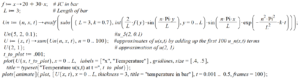
The following Maple code (from the video) no longer seems to work.

 f := x -> 20 + 30*x;
L := 3;
Un := (n, x, t) -> evalf(subs({L = 3, k = 0.7},
  int(2*f(y)*sin(n*Pi*y/L)/L, 
  y = 0 .. L)*sin(n*Pi*x/L)*exp(-n^2*Pi^2*k*t/L^2)));
Un(5, 2, 0.1);
U := (x, t) -> sum(Un(n, x, t), n = 0 .. 100);
U(2, 1);
t_to_plot := 0.001;
plot(U(x, t_to_plot), x = 0 .. L, 
  labels = ["x", "Temperature"],
  gridlines, size = [0.4, 0.5], 
  title = typeset("Temperature u(x,t) at t =", t_to_plot));
plots[animate](plot, [U(x, t), x = 0 .. L, 
  thickness = 3, 
  title = "temperature in bar"], 
  t = 0.001 .. 0.5, frames = 100);

 

Below is a screen capture of the above commands in Maple.

---

---